GOES satellites use L-band (1690-1710MHz, e.g., GOES-18’s 1698MHz downlink at 12Mbps) and S-band (137.9125MHz telemetry) to relay storm imagery, solar X-rays—frequencies optimized for low interference, enabling real-time weather monitoring across the Americas.
Table of Contents
What is the GOES Satellite?
They are positioned in a geostationary orbit, approximately 35,786 kilometers (22,236 miles) above the Earth’s equator. At this exact altitude, a satellite’s orbital period matches the Earth’s rotation rate of 24 hours. This means that from our perspective on the ground, these satellites remain fixed over the same spot on the globe, providing a constant, uninterrupted watch over the same geographic area. The current operational fleet includes GOES-18 (serving as GOES-West at 137.2°W longitude, watching over the western Americas and the Pacific Ocean) and GOES-16 (serving as GOES-East at 75.2°W, monitoring the eastern Americas and the Atlantic Ocean). These satellites are not just cameras in the sky; they are sophisticated data collection platforms with a design life of 15 years, though many exceed this expectancy.
Unlike a low-Earth orbit satellite that circles the planet every 90 minutes, seeing a location for only a few minutes per pass, a GOES satellite can stare at weather systems 24/7. This allows it to create time-lapses of atmospheric phenomena, tracking the development of a thunderstorm from a small cumulus cloud to a powerful mesoscale convective system in real-time. The data collection speed is staggering. The Advanced Baseline Imager (ABI), the main weather instrument on the newest GOES-R series satellites (like GOES-16 and GOES-18), can scan the entire continental United States every 5 minutes. It can even focus on a specific severe weather area, scanning that single sector every 30 to 60 seconds, providing meteorologists with near-real-time data on rapidly evolving events like tornado formation. The ABI doesn’t just take simple pictures; it captures data across 16 different spectral bands, from visible light (with a resolution of 0.5 kilometers per pixel for the “blue” band) to various infrared channels.
| Satellite Series | First Launch | Design Life | Primary Instrument (ABI) Resolution (Visible) | Data Downlink Rate | Notable Improvement |
|---|---|---|---|---|---|
| GOES-R (e.g., GOES-16) | 2016 | 15 Years | 0.5 km | ~100 Mbps | 4x better spatial resolution, 5x faster scanning than previous series |
| GOES-T (e.g., GOES-18) | 2022 | 15 Years | 0.5 km | ~100 Mbps | Improved hardware for better thermal management and reliability |
The information collected by these satellites is not just for tomorrow’s weather forecast. It feeds directly into numerical weather prediction models, improving the accuracy of 3 to 7-day forecasts by up to 15%. It is used for aviation route planning, severe weather warnings for public safety, monitoring volcanic ash plumes for aviation, and tracking sea surface temperatures for hurricane intensity forecasting. The total cost of the GOES-R series program, which includes four satellites (R, S, T, and U), is approximately $10.8 billion, covering their design, build, launch, and operation over their lifetimes.
GOES Frequencies and Their Jobs
The incredible images and data from GOES satellites don’t just magically appear; they travel 22,000 miles to Earth on specific radio frequencies, each chosen for a distinct job. Think of these frequencies as dedicated lanes on a data highway. The GOES-R series satellites, like GOES-16 and GOES-18, primarily transmit their data using three main frequency bands: L-band for downlinking the raw satellite data to ground stations, S-band for satellite control and low-rate data, and a high-powered Ku-band link for broadcasting processed weather data directly to users. The primary downlink for the massive amount of data collected by the Advanced Baseline Imager (ABI) and the Geostationary Lightning Mapper (GLM) occurs in the 1691 MHz and 1701 MHz range within the L-band. This data is sent with a high power of about 50 watts to a small number of NOAA’s primary ground stations, known as the Command and Data Acquisition (CDA) sites. The sheer volume is immense; the satellite generates data at an average rate of about 10 terabits per day, but after on-board processing and compression, the downlink rate to the CDA is approximately 15 to 20 megabits per second (Mbps) per carrier.
For direct broadcast to a wider audience of meteorologists and weather enthusiasts, GOES uses a separate, high-power service called the GOES Rebroadcast (GRB). This is the most important frequency for most data users. GRB is transmitted in the Ku-band, specifically between 1694.1 MHz and 1694.4 MHz for the uplink to the satellite, which then rebroadcasts it down in the 18.3 GHz to 18.8 GHz range. The advantage of GRB is its high Effective Isotropic Radiated Power (EIRP), which can exceed 54 dBW over the continental United States. This high power allows users with relatively small, affordable antennas—as small as 1.8 meters (about 6 feet) in diameter—to receive a complete copy of all the satellite’s core data products with a latency of under 30 seconds. The GRB data stream is a constant flow of information, multiplexing all 16 ABI bands, lightning data, space weather information, and other environmental data streams into a single carrier with a total symbol rate of approximately 2.7 million symbols per second (Msps).
| Frequency Band | Specific Frequencies | Primary Function | Data Rate / Key Parameter | Key User Equipment Needed |
|---|---|---|---|---|
| L-band (Downlink) | 1691 MHz, 1701 MHz | Raw data downlink to NOAA’s primary ground stations (CDA). | ~15-20 Mbps per carrier | Large, professional ground station (≥7m antenna). |
| Ku-band (GOES Rebroadcast – GRB) | Downlink: 18.3 – 18.8 GHz | Direct broadcast of all processed data to public users. | ~2.7 Msps (symbol rate) | 1.8-2.4 meter antenna with Ku-band LNB and a dedicated receiver. |
| S-band (TT&C) | Uplink: ~2092 MHz, Downlink: ~2037 MHz | Satellite command, control, and health telemetry. | ~4 kbps | Exclusive to NOAA satellite operations center. |
| HRIT/EMWIN | 1692.7 MHz (GOES-16) / 1692.9 MHz (GOES-18) | Legacy low-rate data service for text/data and basic imagery. | 128 kbps | Smaller, simpler ~1m antenna and software-defined radio (SDR). |
It’s crucial to distinguish between the legacy data services and the modern GRB. Before the GOES-R series, the primary data service was called GOES VARiable (GVAR), which operated in the 1680-1710 MHz L-band range. While GVAR is now obsolete for the new satellites, many older receiving systems were built for it. The GRB system on the new satellites represents a significant upgrade, providing more than 20 times the data volume of the old GVAR service. For users receiving the data, the signal strength is measured as the G/T ratio (Gain over Temperature) of their receiving system. A typical setup with a 2.4-meter antenna and a low-noise block downconverter (LNB) with a noise figure of 0.5 dB can achieve a G/T of about 22 dB/K, which is sufficient for reliable reception of the GRB signal across most of the satellite’s coverage area. The total cost for a complete personal GRB receiving station, including antenna, mount, LNB, receiver, and computer, can range from 5,000, depending on the component quality and antenna size.
Receiving GOES Satellite Signals
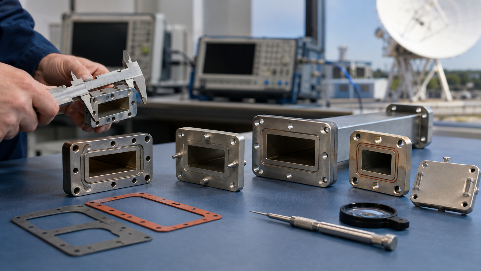
Pulling data directly from a GOES satellite orbiting at an altitude of 35,786 kilometers is an achievable technical project, but it requires specific hardware and precise setup. The process hinges on capturing the satellite’s high-frequency Ku-band GOES Rebroadcast (GRB) signal, which is relatively weak by the time it reaches the Earth’s surface. A complete receiving station consists of four core components: a physically large parabolic antenna (typically 1.8 to 2.4 meters or 6 to 8 feet in diameter) to collect enough signal power, a low-noise block downconverter (LNB) mounted on the antenna to amplify and convert the high-frequency signal, a coaxial cable with low signal loss to connect the antenna to the receiver, and a specialized receiver or software-defined radio (SDR) inside to decode the digital data stream. The total cost for a new, reliable setup typically falls between 4,000, with the antenna and mount representing about 60% of that cost.
A 2.4-meter antenna provides approximately 4 dB more gain than a 1.8-meter antenna. This extra gain is the difference between a stable, 24/7 data flow and a signal that drops out during light rain or cloud cover. The LNB’s quality is measured by its noise figure, with high-quality models rated below 0.7 dB. The LNB is responsible for the first stage of amplification, and a lower noise figure means it adds less inherent interference to the already-weak signal. The LNB also downconverts the high 18 GHz Ku-band signal to a more manageable L-band range, typically around 1350 MHz, which can travel over standard coaxial cable with acceptable loss. For a 30-meter (100-foot) run of RG-6 coaxial cable, the signal attenuation at 1350 MHz is approximately 6 dB, meaning the signal power is reduced to about 25% of its original strength by the time it reaches the receiver.
Proper antenna alignment is not a suggestion; it is an absolute requirement with a tolerance of less than 0.2 degrees. The satellite is a stationary target, but from any point on Earth, it has a specific azimuth (compass direction) and elevation (angle above the horizon). For a receiver in Chicago, Illinois, aiming at the GOES-16 satellite (at 75.2°W longitude) requires pointing the antenna to an azimuth of approximately 142.5 degrees (southeast) and an elevation of about 39.8 degrees above the horizon. An alignment error of just 0.5 degrees can reduce the received signal power by over 3 dB, cutting it in half.
Modern setups often use an SDR like the Airspy R2 or SDRplay RSP1, which, coupled with a computer, replaces a dedicated hardware receiver. The SDR samples the analog signal from the LNB at a high rate—often 2.5 to 3 million samples per second (MS/s)—and converts it into a digital data stream. Software like goestools or SDR# then takes over, locking onto the signal by tuning to the exact center frequency, which for GOES-16 GRB is 1694.1 MHz and for GOES-18 is 1694.9 MHz. The software must also account for the signal’s symbol rate of 2.7 million symbols per second (Msps) and apply error correction. A successful lock is indicated by a low Bit Error Rate (BER), typically better than 1 error in 10^6 bits.
Equipment for Capturing GOES Data
Building a ground station to capture data directly from the GOES satellite requires a specific set of components that work together to receive a weak signal from 36,000 kilometers away. The system’s success depends on each link in the chain. The core components you will need to acquire are:
- A parabolic antenna, ideally 1.8 meters (6 feet) or larger in diameter.
- A feedhorn and Low-Noise Block Downconverter (LNB) with a noise figure below 0.7 dB.
- Low-loss coaxial cable, such as QR-540 or LMR-400, with a maximum length of 30 meters (100 feet).
- A mounting pole and robust hardware to ensure absolute stability in winds exceeding 80 km/h (50 mph).
- A software-defined radio (SDR) receiver like the Airspy R2 (~$200 USD) or SDRplay RSP1.
- A dedicated computer, such as a Raspberry Pi 4 (~$75 USD) or a standard desktop PC, running decoding software.
A 2.4-meter antenna provides a gain of approximately 39.5 dBi at the GOES downlink frequency of 1.7 GHz, while a smaller 1.8-meter dish offers about 35.5 dBi. This 4 dBi difference represents a 60% increase in effective signal capture area. The antenna’s surface accuracy is paramount; a peak-to-peak deviation of more than 3 mm across the reflector will scatter the signal and drastically reduce performance. The antenna must be mounted on a perfectly rigid pole with a diameter of at least 5-7 cm (2-3 inches), using galvanized steel U-bolts. The entire assembly must be plumb, with less than 1 degree of deviation from vertical, to allow for accurate satellite targeting.
The feedhorn must be positioned at the exact focal length, which for a standard offset dish is typically 45-50% of the dish’s height from the bottom. The LNB’s local oscillator (LO) frequency is 10750 MHz, which converts the incoming 1694.1 MHz GRB signal down to an intermediate frequency (IF) of 1350 MHz that travels efficiently over the coaxial cable. The LNB’s noise figure is more critical than its gain; an LNB with a 0.5 dB noise figure will outperform one with a 1.0 dB noise figure and higher gain, because it adds less inherent electronic noise to the weak signal. The coaxial cable connecting the LNB to the indoor receiver is a major source of signal loss. Standard RG-6 cable has an attenuation of about 6.5 dB per 30 meters at 1350 MHz, meaning over half the signal power is lost. Using a lower-loss cable like LMR-400, which has an attenuation of only 3.5 dB per 30 meters, can be the difference between a marginal and a robust signal lock.
Turning Signal Data into Images
The data you receive isn’t a simple picture file; it’s a multiplexed packet stream containing calibrated sensor measurements for millions of individual points. The transformation requires specific software to unpack, calibrate, and render this data. The key stages handled by software like goestools or Xrit-Rx are:
- Demodulation and Decoding: Locking onto the 2.7 megabaud signal and applying Viterbi and Reed-Solomon error correction to produce a clean data stream.
- Demultiplexing: Separating the single stream into individual files for each of the ABI’s 16 spectral bands and other data products like the Geostationary Lightning Mapper (GLM).
- Calibration: Applying mathematical formulas to convert the sensor’s 10-bit or 12-bit digital numbers into scientifically meaningful values like reflectance or brightness temperature.
- Mapping and Projection: Stretching the data to fit a standard map projection, correcting for the satellite’s viewing angle.
- Enhancement and Coloring: Applying color palettes to highlight specific features, like severe weather or atmospheric moisture.
The first software, typically a Virtual Instrument Software Architecture (VISA) decoder, processes the ~2.7 million symbols per second stream. It corrects for phase shifts and applies forward error correction (FEC), which can recover a usable signal even with a Bit Error Rate (BER) as high as 1×10^-3. A successful decode results in a continuous flow of data packets. A demultiplexer, such as the goesrecvprogram, then sorts these packets. Each packet has a header specifying its Application ID (APID), which identifies it as, for example, ABI Band 2 (Visible, 0.64 µm) or Band 13 (Clean IR, 10.3 µm). The demultiplexer saves the data for each APID into separate files, often using the HRIT (High Rate Information Transmission) or LRIT (Low Rate Information Transmission) file format. A single full-disk image scan from the ABI, which captures over 700 million pixels per band, results in a file size of approximately 15-25 megabytes per spectral band.
For the visible bands (Bands 1-6), this means converting the sensor’s raw count into reflectance factor, a unitless ratio from 0 (total absorption) to 1 (total reflection). The calibration formula involves multiplying the digital number by a gain factor (around 0.00002) and adding an offset (around -0.2). For the infrared bands (Bands 7-16), the process converts the raw data into brightness temperature in Kelvin, using a complex quadratic formula with coefficients provided by NOAA. The difference in resolution is significant; the 2 km resolution IR bands have approximately 5,000 x 3,000 pixels per full disk image, while the 0.5 km resolution visible band has about 20,000 x 12,000 pixels.
GOES Data in Everyday Use
The value of GOES data is measured not in gigabytes downloaded, but in the tangible decisions it enables across dozens of industries. The satellite’s 24/7 stream of information flows directly into systems that affect everything from your morning commute to the price of food. The data’s application spans multiple critical sectors:
| Application Area | Key GOES Data Used | Impact Metric | Primary Users |
|---|---|---|---|
| Weather Forecasting & Warnings | ABI Bands 8-16 (IR), Band 13 (Clean IR), GLM | +40% accuracy in 3-day hurricane track forecasts; tornado warning lead time now avg. 18 min (up from 10 min in 2000). | National Weather Service, Media Meteorologists |
| Aviation & Transportation | ABI Band 2 (0.64µm Visible), Band 13 (10.3µm IR) | ~$150 million annually saved in optimized flight routes per major airline; reduces delays at hubs like ATL/ORD by ~8%. | Airlines, FAA, Dispatchers |
| Agriculture & Water Management | ABI Band 6 (2.2µm Veggie), Band 13 (10.3µm IR) | Improves irrigation efficiency by ~15%; crop yield forecasts within ±3% accuracy 3 months before harvest. | Farmers, Agronomists, Water Districts |
| Energy Sector | ABI Band 5 (1.6µm Cloud Particle), Band 7 (3.9µm Shortwave IR) | Manages ~5 GW of solar power load on grid; predicts cloud cover impact on output with 92% accuracy for 6-hour forecasts. | Utility Companies, Power Traders |
| Disaster Response | ABI Band 7 (3.9µm Fire Hotspot), Band 6 (2.2µm Smoke) | Detects wildfires as small as 10 acres (4 hectares); monitors volcanic ash plumes for aviation safety within 5 min of eruption. | Emergency Managers, US Forest Service |
The most immediate use is in high-resolution numerical weather prediction (NWP) models. Forecast models like the Global Forecast System (GFS) and the High-Resolution Rapid Refresh (HRRR) assimilate over 5 million GOES ABI observations every 6 hours. These data points, especially from the water vapor channels (Bands 8-10), provide a 3D map of atmospheric moisture and wind vectors, initializing the model with real-world conditions. This data injection has improved the accuracy of 48-hour precipitation forecasts by approximately 12% since the GOES-R series became operational. For severe weather, the Geostationary Lightning Mapper (GLM) provides a total lightning density measurement. A sudden 50% increase in flash rate inside a thunderstorm is a reliable indicator of intensification, giving forecasters a crucial 10 to 15 minutes of extra lead time to issue tornado or severe thunderstorm warnings.
Pilots use 1-minute “mesoscale” sector scans of Band 13 (clean IR) to identify the altitude and temperature of thunderstorm tops. Avoiding the coldest cloud tops (below -60°C) helps prevent turbulence and hail damage, reducing flight diversions by an estimated 5% annually. For agriculture, the 0.5 km resolution visible bands are used to calculate the Normalized Difference Vegetation Index (NDVI), a measure of plant health. A farmer can monitor a field’s NDVI value, which ranges from -0.1 (bare soil) to +0.9 (dense vegetation), and identify areas of stress with a 10-meter spatial accuracy, allowing for precise application of water and fertilizer. This precision agriculture can reduce fertilizer costs by 20 per acre on a 5,000-acre farm.