Log Periodic Antenna Working Principle Explained | Broadband, Self-Similar Structure

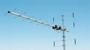
A log-periodic dipole array (LPDA) uses progressively shorter dipoles and a common feed line to cover a broad frequency range. As frequency rises, the strongest radiating currents move toward the shorter elements. The antenna can therefore work across several bands without changing its physical length. Its usable bandwidth still depends on the finished design and measured performance.^[1]

How the active region moves

The feed normally enters at the short-element end. Adjacent dipoles connect to opposite sides of the balanced feed line, reversing the connection from one element to the next. The feed-line phase delay and coupling between elements also affect their currents; the array does not operate as a set of isolated dipoles.

At a given frequency, elements near half a wavelength carry much of the radiating current. This group is the active region. Higher frequencies use shorter wavelengths, so the active region shifts toward the smaller end. At lower frequencies it moves toward the larger end. Elements outside that region still interact with the array; they are not electrically invisible.^[2]

The main beam of a conventional end-fire LPDA points toward the shorter elements. Mounting the antenna in the correct direction and polarization remains necessary. Broadband operation does not make a directional antenna omnidirectional.

A numerical example: frequency and element length

For a first free-space estimate, wavelength in metres is approximately 300 ÷ frequency in MHz. Half that wavelength gives an initial estimate of a dipole’s full tip-to-tip length.

Frequency	Approximate wavelength	Half-wave length
100 MHz	3.00 m	1.50 m
200 MHz	1.50 m	0.75 m
400 MHz	0.75 m	0.375 m

These are calculated scale estimates, not fabrication dimensions. Element diameter, end effects, the feed structure and mutual coupling change the required physical lengths. A printed antenna also depends on its substrate.

Moving from 100 to 400 MHz is a 4:1 frequency ratio. A 30 MHz–3 GHz claim represents 100:1, not 10:1. Treat either bandwidth claim as a specification to verify from gain, pattern and impedance data for the particular antenna.

Why the structure is called log-periodic

Number the elements from longest to shortest and define τ = L_n+1 / L_n, with 0 < τ < 1. In the ideal scaled structure, successive lengths and spacings shrink by the same factor. The electrical behavior repeats approximately when frequency changes by the corresponding ratio.^[3]

For a calculated example with τ = 0.85, three successive lengths are 2.000 m, 1.700 m and 1.445 m. Their approximate resonant frequencies rise by a factor of 1/0.85, or about 1.176, at each step. The ratio 0.85 is an example, not a universal design setting.

A real antenna has a finite number of elements. Once the active region reaches either end, it no longer sees the same surrounding structure. That is one reason the operating band cannot be inferred from the longest-to-shortest length ratio alone.

For a purely geometric length ratio of 10:1 and τ = 0.85, the relation 0.85^N−1 ≤ 0.1 requires at least 16 elements. That calculation counts geometric steps; it does not prove a 10:1 usable RF bandwidth or a particular gain.

Tau, spacing and apex angle

Use one length convention throughout a drawing. Here L is the full tip-to-tip dipole length, d is the distance to the next shorter element along the boom, and α is the angle between the boom axis and the line through the element tips.

• Scaling factor: τ = L_n+1 / L_n.
• Spacing factor: σ = d_n / (2L_n).
• Half-apex angle: α = arctan[(1 − τ)/(4σ)]. The full included angle is 2α.

These definitions connect the element lengths, separation and taper; they do not independently specify the antenna’s gain.^[4]

With τ = 0.90 and σ = 0.15, α is about 9.46° and the full included angle is about 18.92°. For a 1.00 m element, the next spacing is 2 × 0.15 × 1.00 = 0.30 m. Increasing σ while keeping τ fixed makes the taper angle smaller.

A τ value closer to 1 requires more elements to span the same geometric length ratio. Designers must then balance boom length, spacing, feed impedance and the required radiation pattern. A single τ-to-gain lookup cannot replace analysis of the complete antenna.

What VSWR tells you—and what it does not

VSWR describes the impedance match at a stated reference plane and system impedance. For VSWR S, the reflection-coefficient magnitude is |Γ| = (S − 1)/(S + 1). The reflected fraction of incident power is |Γ|²; mismatch loss is −10 log₁₀(1 − |Γ|²).^[4]

VSWR	Reflected power	Mismatch loss
1.5:1	4.0%	0.18 dB
2:1	11.1%	0.51 dB
3:1	25.0%	1.25 dB

These calculated values describe mismatch at one interface. They exclude cable and conductor losses. Reflected power is not automatically converted into heat in the cable, and the power accepted by the antenna is not necessarily all radiated.

A good VSWR curve alone does not prove useful gain, correct polarization or a clean beam. A resistive load can have an excellent impedance match without acting as an efficient antenna. Specify 50 Ω or 75 Ω explicitly; an LPDA does not automatically match both systems.

Gain, beam direction and reception

A passive antenna concentrates radiation in some directions at the expense of others. It does not supply amplifier power. A gain of 7 dBi corresponds to about 5.0 times the radiation intensity of an isotropic reference in the stated direction for equal accepted power; it is not a fivefold improvement in every received signal.

Compare gain values at the same frequency and check whether they are gain or realized gain. Realized gain includes input mismatch. Cable loss, polarization mismatch, pointing and obstructions still affect the signal reaching the receiver.

For example, a stated realized gain of 7 dBi followed by a cable with 2 dB loss leaves about 5 dBi before other link losses. Increasing antenna gain will not remove a blockage or guarantee reception at a specified distance.

LPDA, Yagi and waveguide horn: different choices

An LPDA feeds all its dipoles through a common line. A conventional Yagi-Uda uses a driven element with parasitic directors and a reflector. Compare actual bandwidth and pattern requirements before choosing either; a narrowband link and a wide frequency sweep ask different things of an antenna.

A waveguide horn uses a flared aperture, so an LPDA and a horn are not interchangeable labels. In microwave measurements, a standard gain horn may serve as a reference when its frequency range, calibration and polarization fit the setup. A quad-ridged antenna uses another broadband geometry; compare its port arrangement and polarization data with the required measurement.

How to check a proposed antenna

1. Write down both band edges. Include required transmit and receive bands, not only a center frequency.
2. Ask for full-band plots. Review VSWR, realized gain and front-to-back ratio, including any dips between plotted sample frequencies.
3. Check patterns and polarization. Request principal-plane patterns at the low, middle and high parts of the band, plus frequencies where performance changes sharply.
4. Define the measurement setup. Record the reference plane, cable corrections, antenna separation, mounting and calibration information. Separate measured results from simulation.
5. Check installation limits. Confirm connector access, mounting loads, wind and ice requirements, corrosion protection and any transmitter power limit for the actual model.

Published research illustrates why several measurements are needed: Mistry and colleagues studied a ten-element LPDA over 470–860 MHz and compared simulated and measured realized gain, while optimizing VSWR and front-to-back ratio separately. Those results apply to that study’s design; they are not test data for a Dolph product.^[4]