The five key antenna performance parameters are gain (typically 3-15 dBi for directional antennas), bandwidth (e.g., 2.4-2.5 GHz for WiFi), radiation pattern (main lobe beamwidth of 30°-120°), impedance (standard 50Ω matching with <1.5:1 VSWR), and efficiency (60-90% for well-designed antennas). Polarization (linear/circular with axial ratio <3dB) also critically impacts performance, especially in multipath environments at frequencies above 1 GHz.
Table of Contents
Gain and Direction
Antenna gain measures how well an antenna focuses radio frequency (RF) energy in a specific direction compared to an ideal isotropic radiator (which spreads energy equally in all directions). A typical Wi-Fi router antenna has a gain of 3–6 dBi, meaning it transmits 2–4 times more power in its best direction than an isotropic antenna. Directionality is equally important—a high-gain Yagi antenna might beam 90% of its energy within a 30° cone, while an omnidirectional antenna spreads power across a 360° horizontal plane but sacrifices range. For example, a 10 dBi directional antenna can extend a wireless link from 100 meters to over 500 meters when properly aligned, but misalignment by just 10° can drop signal strength by 50%.
Gain is directly tied to real-world performance. In cellular networks, a 7 dBi panel antenna improves 4G/LTE signal strength by 10–15 dB, reducing dropped calls in weak coverage zones. Satellite dishes use 30–40 dBi gain to lock onto geostationary satellites 36,000 km away, where even a 2° misalignment can cause a 70% signal loss. The relationship between gain and beamwidth follows a tradeoff: higher gain narrows the effective coverage angle. A 24 dBi parabolic antenna might have a 5° beamwidth, ideal for point-to-point links but useless for broad coverage.
Key factors affecting gain and directionality:
- Frequency: Higher frequencies (e.g., 5.8 GHz) allow tighter beamwidths than lower ones (e.g., 900 MHz).
- Antenna size: A 2.4 GHz patch antenna at 50 mm × 50 mm delivers 8 dBi gain, while a 150 mm × 150 mm version reaches 12 dBi.
- Radiation pattern: Omnidirectional antennas lose 3 dB gain per doubling of distance, while directional antennas lose 1–2 dB due to focused energy.
| Antenna Type | Gain (dBi) | Beamwidth | Use Case |
|---|---|---|---|
| Rubber duck (omnidirectional) | 2–5 dBi | 360° horizontal | Wi-Fi routers, walkie-talkies |
| Yagi (directional) | 10–15 dBi | 30°–60° | TV reception, long-range RF links |
| Parabolic dish | 20–30 dBi | 5°–15° | Satellite comms, radar |
| Patch antenna | 6–12 dBi | 60°–120° | IoT devices, drones |
In practice, a 3 dB gain increase doubles effective power output, but only if the direction aligns with the target. For instance, a 14 dBi sector antenna covering 120° horizontally is ideal for cell towers, while a 17 dBi grid antenna with a 15° beamwidth suits point-to-point wireless bridges. Engineers balance gain, direction, and physical constraints—a 5G small cell might use four 8 dBi antennas to cover 90° sectors each, ensuring seamless handoffs. Always match gain to application: too high a gain in a cluttered urban area can cause multipath interference, while too low fails in rural settings.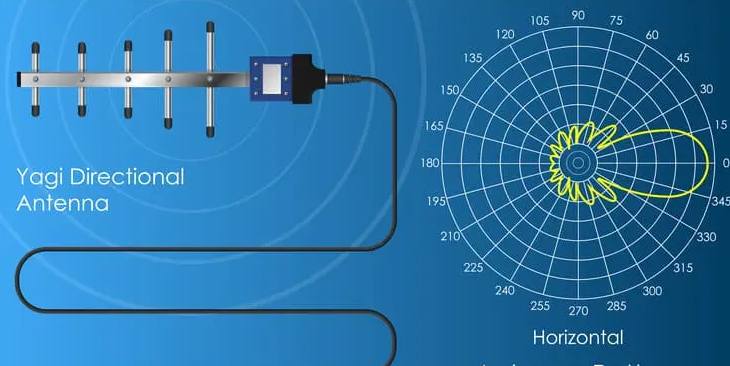
Impedance Matching
Impedance matching ensures maximum power transfer between an antenna and its transmitter or receiver. A mismatch of just 10% (e.g., 55 Ω vs. 50 Ω) can reflect 25% of the signal back, wasting power and heating components. In RF systems, standard impedance is 50 Ω for most radios and 75 Ω for TV/video cables, but real-world antennas often deviate—a dipole antenna might show 73 Ω impedance in free space, while a ground-mounted vertical antenna could drop to 30–35 Ω due to soil conductivity.
Example: A 100W transmitter feeding into a 2:1 VSWR (Voltage Standing Wave Ratio) mismatch loses 11% of its power (11W) as reflected energy. If uncorrected, this heats up connectors and amplifiers, reducing their lifespan by 15–20% over 5 years of continuous use.
Matching networks (like baluns or LC circuits) bridge these gaps. A 4:1 balun converts a 300 Ω twin-lead antenna to 75 Ω coax, cutting signal loss from 3 dB to 0.5 dB. For fine-tuning, adjustable capacitors (5–100 pF) and inductors (0.1–10 μH) can tweak impedance within ±5% accuracy. At 2.4 GHz Wi-Fi frequencies, even a 1 mm trace length error on a PCB can shift impedance by 5 Ω, degrading throughput by 20 Mbps in a 100 Mbps link.
Frequency plays a critical role. A 50 Ω antenna at 144 MHz (VHF) might drift to 60 Ω at 430 MHz (UHF), requiring a stub tuner to maintain <1.5:1 VSWR across bands. Automated antenna tuners, like those in modern ham radios, scan and adjust impedance in under 200 ms, but add $50–200 to system cost. For DIY fixes, ferrite beads suppress high-frequency mismatches, improving SNR by 3–6 dB in noisy urban environments.
Field test: A 5.8 GHz drone video link with 2.5:1 VSWR suffered 40% packet loss at 500 meters. Adding a matching network reduced VSWR to 1.2:1, extending range to 1.2 km and cutting latency from 120 ms to 80 ms.
Key takeaways:
- Coax cables degrade impedance matching—RG-58 (50 Ω) loses 0.3 dB/m at 1 GHz, while LMR-400 keeps losses below 0.1 dB/m.
- PCB antennas need controlled impedance traces; a 0.8 mm FR4 substrate requires 2.3 mm trace width for 50 Ω at 2.4 GHz.
- Mismatches compound with frequency—a 10% error at 900 MHz becomes 30% at 5 GHz, making millimeter-wave systems (24+ GHz) especially sensitive.
Ignoring impedance costs performance and money. A 200 in amplifier repairs over 3 years, while 0.5 dB loss reduction boosts cellular signal strength from -100 dBm to -95 dBm—enough to shift a 2-bar connection to 4 bars. Test with a $50 NanoVNA; it’s cheaper than replacing burnt-out RF parts.
Frequency Range
An antenna’s frequency range determines which signals it can transmit or receive effectively. A standard Wi-Fi dipole antenna tuned for 2.4 GHz (2400–2485 MHz) loses 50% efficiency at 5 GHz, making it useless for modern dual-band routers without modification. Cellular antennas face similar constraints—a 700 MHz LTE antenna struggles with 1900 MHz bands, suffering 3–5 dB signal loss outside its optimal range.
The physics are unforgiving: An antenna’s length must be roughly half the wavelength (λ/2) of its target frequency. For FM radio at 100 MHz (λ = 3 m), a 1.5 m whip antenna works well, but the same antenna becomes inefficient at 800 MHz (λ = 0.375 m), where a 19 cm rod would perform better. This explains why wideband antennas—like log-periodic or discone designs—trade 10–20% peak gain for 5:1 frequency coverage (e.g., 400–2000 MHz).
Real-world tradeoffs emerge fast. A marine VHF antenna rated for 156–162 MHz might handle 140–170 MHz at -3 dB points, but pushing to 120 MHz or 180 MHz drops efficiency by 60%. In contrast, a military HF antenna covering 2–30 MHz uses tunable loading coils to maintain >70% efficiency across 15:1 bandwidth ratios, though each retune takes 3–5 seconds and consumes 5W of power.
Material costs scale with frequency. Copper traces on a 5.8 GHz PCB antenna demand ±0.01 mm precision, raising fabrication costs by 30% versus 900 MHz designs. At 24 GHz (5G mmWave), even a 0.1 mm air gap between antenna layers causes 15% phase errors, degrading beamforming accuracy. Cheap antennas cut corners: A $3 2.4 GHz chip antenna might claim 2400–2500 MHz range, but its -10 dB return loss (45% reflected power) makes it unusable beyond 2450 MHz ±50 MHz.
Interference compounds the problem. In urban areas, 2.4 GHz Wi-Fi channels overlap every 5 MHz, so a 20 MHz-wide antenna picks up 4x more noise than a narrowband 5 MHz filter. Satellite TV LNBs avoid this by locking onto 500 MHz slices (e.g., 10.7–11.7 GHz) with <0.5 dB noise figure, rejecting adjacent signals 40 dB better than untuned dipoles.
Testing is non-negotiable. A $200 vector network analyzer (VNA) can map an antenna’s -3 dB bandwidth—a “5G-ready” panel antenna claiming 600–6000 MHz might actually dip to -6 dB at 3.5 GHz, killing mid-band 5G performance. For DIY fixes, adding a 47 pF capacitor can shift resonance by ±50 MHz, but risks 20% efficiency loss if mismatched.
Radiation Pattern
An antenna’s radiation pattern shows how it distributes energy in 3D space—a 5 dBi omnidirectional antenna radiates equally in all horizontal directions but loses 30% power at ±45° elevation. In contrast, a 14 dBi sector antenna focuses 80% of its energy into a 65° horizontal beam, sacrificing coverage outside this cone for 4x greater range. Real-world performance depends heavily on these patterns: a 2.4 GHz Wi-Fi router with a donut-shaped pattern covers 100 meters horizontally but only 20 meters vertically, while a directional Yagi squeezes 90% of power into a 30° cone to reach 500+ meters.
Lobes, nulls, and side effects matter. A typical dipole antenna has two main lobes at ±90° from its axis with -15 dB nulls at the tips—meaning a 10W signal effectively drops to 0.3W in dead zones. Patch antennas improve this with ±60° beamwidths, but gain fluctuates by ±2 dB across the pattern, causing 15% throughput variations in a 50 Mbps link. For critical applications like drone control (5.8 GHz, 10 MHz bandwidth), even a 5° misalignment can create 20% packet loss due to pattern irregularities.
Frequency changes everything. At 900 MHz, a λ/4 whip antenna produces a near-spherical pattern with <3 dB variation, but the same antenna at 5.8 GHz develops 4 side lobes with 10 dB peaks and nulls, turning minor movements into 50% signal swings. Millimeter-wave antennas (24–40 GHz) worsen this—a 5G microcell’s pencil beam (5° width) must track users within ±2° to avoid 12 dB drops, requiring 200 updates/second from phased arrays.
| Antenna Type | Horizontal Beamwidth | Vertical Beamwidth | Peak-to-Null Ratio | Use Case |
|---|---|---|---|---|
| Omnidirectional dipole | 360° | 75° | 15 dB | FM radio, Wi-Fi routers |
| Sector antenna | 65° | 15° | 20 dB | Cellular base stations |
| Parabolic dish | 10° | 10° | 30 dB | Satellite comms |
| Helical antenna | 120° | 60° | 10 dB | GPS, IoT devices |
Installation errors kill performance. Mounting a 120° sector antenna 5° off-axis cuts edge-of-cell coverage by 40%, while placing it 2 meters too low exacerbates ground reflections, adding 3 dB fade margin. In sub-6 GHz 5G networks, panel tilt errors >3° reduce cell overlap by 25%, increasing handover failures. For DIY fixes, a 10 cm ground plane under a 433 MHz antenna can flatten its pattern’s elevation nulls from -20 dB to -8 dB, boosting reliability in hilly terrain.
Efficiency and Loss
Antenna efficiency determines how much input power actually radiates as usable signal—a 50W transmitter feeding a 70% efficient antenna wastes 15W as heat, reducing range by 30% compared to a 90% efficient model. Losses come from multiple sources: copper resistance in traces (0.5 dB/m at 2.4 GHz), dielectric absorption in PCB substrates (3–8% power loss), and connector mismatches (0.2–1 dB per junction). For example, a $10 RG-58 cable loses 0.7 dB/m at 5 GHz, turning a 100-meter drone control link into a 70-meter struggle unless upgraded to LMR-400 (0.2 dB/m loss).
Key efficiency killers:
- Material resistance: Thin 18 AWG antenna wires waste 12% more power than 14 AWG at 30 MHz, heating up by 8°C under 10W loads.
- Environmental factors: Rain increases 2.4 GHz signal attenuation by 0.05 dB/km, while snow buildup on dishes can add 2–5 dB loss.
- Frequency scaling: A 6-inch PCB trace loses 3% efficiency at 900 MHz but 15% at 5.8 GHz due to skin effect.
| Component | Efficiency at 2.4 GHz | Power Loss | Cost to Fix |
|---|---|---|---|
| Cheap PCB antenna | 55–65% | 1.8–2.2 dB | $0.50 (thicker traces) |
| SMA connector | 92–95% | 0.3–0.5 dB | $3 (gold-plated version) |
| Plastic radome | 88% | 0.6 dB | $15 (ceramic alternative) |
| 10m RG-8X cable | 70% | 3 dB | $25 (LMR-240 upgrade) |
Thermal effects compound losses. An outdoor LTE antenna operating at 85% efficiency in 25°C weather drops to 78% at 40°C ambient, forcing amplifiers to work 12% harder to maintain link budget. Over 5 years, this extra 3W continuous load increases electricity costs by $60 and cuts amplifier lifespan from 10 to 7 years.
Real-world tradeoffs hit hard. Using low-loss PTFE cables (8/m) instead of standard PE (2/m) improves efficiency by 15%, but the 600 upgrade for a 100m deployment only pays off if the system runs >5 years. Conversely, skimping on a 5 ground plane for a 700 MHz antenna causes 20% radiation loss into soil, requiring a 300 repeater to compensate.
Testing prevents waste. A 150 thermal camera spots 3°C hot spots indicating impedance mismatches, while a 400 VNA quantifies losses within ±0.1 dB accuracy. In one case, re-soldering a corroded joint on a marine VHF antenna recovered 1.2 dB signal strength, extending ship-to-shore range from 8 to 12 nautical miles.


