Antenna equipment primarily includes radiating elements (e.g., 20mm×20mm microstrip patches for 2.4GHz operation), feeding networks (RG-58 coaxial cables with 50Ω impedance, <0.5dB/10m loss at 1GHz), matching circuits (π-type networks using 10nH inductors and 10pF capacitors for impedance tuning), and enclosure/support structures (aluminum alloy with 237W/m·K thermal conductivity, IP67-rated for dust/water resistance).
Table of Contents
Metal Radiator Structure
A half-wave dipole for the 2.4 GHz Wi-Fi band has each of its two elements precisely cut to approximately 30.5 mm, resulting in a total length of about 61 mm. A deviation in length of just ±2% can detune the antenna, shifting its resonant frequency by ~50 MHz and increasing the Voltage Standing Wave Ratio (VSWR) to above 1.5:1, which leads to a >10% loss in transmitted power. The material choice is equally critical; high-conductivity metals like copper (with a conductivity of 5.96×10⁷ S/m) or aluminum (3.5×10⁷ S/m) are standard. The cross-sectional thickness, often a 2 mm diameter for wire dipoles or a 35 μm copper layer on PCB antennas, is a trade-off between mechanical strength, weight, and electrical performance—thicker elements exhibit a wider operational bandwidth, often by >15%.
| Parameter | Impact on Performance | Typical Values & Examples |
|---|---|---|
| Length | Determines resonant frequency. | 2.4 GHz dipole: ~61 mm; 900 MHz dipole: ~166 mm. |
| Material & Conductivity | Affects resistive (Ohmic) losses and efficiency. | Copper (~96% IACS), Aluminum (~61% IACS). |
| Element Diameter/Thickness | Influences bandwidth (BW). | A 10 mm tube offers ~12% BW vs. ~7% for a 2 mm wire. |
| Shape/Geometry | Controls directivity and gain. | A parabolic reflector can achieve gains exceeding 24 dBi. |
A straight wire dipole produces a characteristic omnidirectional pattern in the horizontal plane with a ~360-degree coverage but a narrower 75-degree vertical beamwidth. To focus energy and increase gain, more complex shapes like a Yagi-Uda array are employed. Adding 4 parasitic elements (1 reflector and 3 directors) to a driven element can narrow the beamwidth to under 50 degrees and provide a forward gain of 9 to 12 dBi, effectively concentrating ~8x more power in a specific direction compared to a simple dipole. The surface quality is a often-overlooked factor; a smooth, well-plated surface (e.g., with 3-5 μm of silver) minimizes surface resistance and subsequent signal loss.
Corrosion or surface imperfections can increase this resistance, leading to losses that can easily exceed 15% of the input power, especially at frequencies above 1 GHz. For structural elements, aluminum alloys like 6061 are frequently chosen for their favorable strength-to-weight ratio (310 MPa tensile strength) and good corrosion resistance, striking a balance between a 15-year outdoor lifespan and manufacturing cost, which can be ~30% lower than an equivalent stainless steel structure.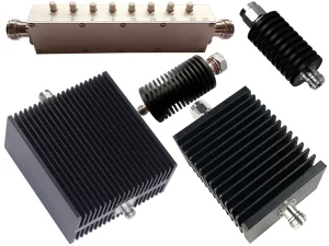
Signal Feed Cable
Unlike standard electrical wire, a coaxial cable is engineered to shield the inner signal and maintain a constant 50-ohm impedance. However, it is not a perfect conductor; signal attenuation is its primary drawback. This loss, measured in decibels per meter (dB/m), is not linear but increases dramatically with frequency. For example, common RG-58 cable suffers a loss of about 0.66 dB/m at 1 GHz. This means over a 15-meter run, you’d lose ~90% of your power before it even reaches the antenna. Higher-quality cables like LMR-400 are far more efficient, with a specified loss of only 0.22 dB/10 ft (3.05 m) at 2.4 GHz, making them essential for longer runs or higher-frequency applications like 5 GHz Wi-Fi or cellular boosters.
| Parameter | Impact & Example Data | Common Specification Range |
|---|---|---|
| Impedance | Must match system (50 Ω for most telecom/wifi). Mismatch causes reflected power (VSWR >1.5:1). | 50 Ω or 75 Ω (video). |
| Attenuation/Loss | Signal loss per unit length. Increases with frequency. | RG-58: 6.9 dB/10m@1 GHz; LMR-400: 2.2 dB/[email protected] GHz |
| Shield Effectiveness | Blocks external interference. Measured in dB of rejection. | Braid: >90% coverage; Foil + Braid: >100 dB rejection. |
| Diameter | Rough indicator of loss and flexibility. | RG-58: ~5 mm; LMR-400: ~10.3 mm. |
The fundamental choice is between a thinner, more flexible cable with higher loss (e.g., RG-58 at ~2.50/meter). The dielectric material separating the inner conductor from the outer shield is a key differentiator; cheaper cables use polyethylene (PE) with a velocity of propagation (VP) of ~66%, meaning signals travel at 66% the speed of light, while more advanced foamed polyethylene (FP) can achieve a VP of ~88%, reducing latency and slightly improving efficiency. The outer shield’s construction is paramount for noise immunity. A simple braided copper shield (e.g., 90% coverage) is good, but a combination of foil plus a braid is superior, providing >100 dB of effective shielding against external electromagnetic interference (EMI), which is crucial in urban environments saturated with RF noise.
Every connection point, typically via N-type or SMA connectors, introduces a small but measurable loss of 0.1 to 0.3 dB each. Therefore, a single uninterrupted cable run is always preferable to multiple segments joined with connectors. The minimum bend radius (e.g., 50 mm for LMR-400) is a critical mechanical specification; exceeding it deforms the internal geometry, altering the impedance and creating signal reflections that can degrade system VSWR by over 15%. For a 25-meter run at 2.4 GHz, using LMR-400 instead of RG-8X can save over 3 dB of loss, which effectively doubles the radiated power output.
Impedance Matching Unit
The impedance matching unit is an essential circuit that ensures maximum power transfer from the transmitter (typically 50 Ω) to the antenna radiator, which can have a vastly different native impedance. Without this critical component, mismatch losses can easily exceed 20-30% of your output power, reflecting energy back into the transmitter and potentially causing damage. For instance, a quarter-wave monopole over a ground plane has a theoretical impedance of 36.5 Ω, directly connected to a 50 Ω cable results in a VSWR of ~1.4:1 and a ~4% power loss. In real-world multi-element arrays, the impedance can be even lower, such as 20-30 Ω, which would create a VSWR above 2.0:1 and dissipate over 10% of the power as heat in the amplifier. Effective matching brings the VSWR down to 1.2:1 or better, reducing reflected power to under 1% and ensuring >99% of your DC power is converted into effective radiated signal.
- Balun (Balanced-to-Unbalanced): A 1:1 current balun made with 10-15 turns of coaxial cable on a FT-240-43 ferrite core can handle >1 kW of power from 1.8 MHz to 30 MHz, suppressing common-mode currents by >30 dB.
- Gamma Match: Common on Yagi antennas, this single-capacitor match uses a 10-20 mm diameter rod and a sliding clamp to adjust capacitance, typically tuning for a < 2% loss across a 5-10% bandwidth around 144 MHz.
- LC Network: A simple $2 kit with an air variable capacitor (5-100 pF) and a 1-2 μH inductor can match a 500 Ω dipole impedance to 50 Ω across the 7 MHz amateur band with < 0.5 dB insertion loss.
- Antenna Tuner: A manual tuner with 3-4 variable capacitors and inductors can force a match on antennas with VSWR up to 10:1, but introduces ~15% loss (about 0.7 dB) even when optimally adjusted.
A low-pass L-network, one of the most common configurations, uses a series inductor (~0.1 μH for 28 MHz operation) and a shunt capacitor (~30 pF) to match a 50 Ω source to a 100 Ω load with a resulting circuit Q factor of ~5 and a operational bandwidth of roughly ±1.5 MHz. The physical construction of these components directly impacts performance and power handling. A capacitor with a 2 mm spacing between its plates might arc over at ~800 V, limiting transmit power to about 500 W PEP, while a premium vacuum variable capacitor with a 10 mm gap can handle >8 kV and 5 kW continuous output.
For permanent installations, a transmission line transformer made with 6-8 turns of bifilar wound 14 AWG wire on a 2.4 cm diameter toroidal core provides a rugged 4:1 impedance transformation (e.g., 200 Ω to 50 Ω) with a remarkable bandwidth from 3 MHz to >50 MHz and an efficiency consistently >95%. The choice between a simple, fixed LC circuit costing <5 and an automatic antenna tuner costing >200 hinges on required bandwidth and operational flexibility; the fixed circuit might cover a single 200 kHz wide band perfectly, while the automatic tuner can force a match across 1.8 MHz to 30 MHz instantly, albeit with an additional 10-15% system loss.
Mounting and Housing Parts
A typical 6-foot VHF antenna array, with a surface area of ~0.5 m², can experience a wind load force exceeding 200 Newtons (N) in a 60 mph (27 m/s) storm. Without a mast and brackets rated for this >20 kg of horizontal force, the entire installation is at risk. Housing materials are equally specialized; a common radome is molded from 3 mm thick UV-stabilized polycarbonate, which attenuates signal by less than 0.2 dB while protecting internal electronics from rain, UV radiation, and temperature swings from -40°C to +85°C. The choice of mast material is a direct trade-off between cost and performance; a 2-inch (50 mm) diameter galvanized steel mast might cost $50 per 10-foot section and support >100 kg, but a lighter 6061-T6 aluminum mast of the same size, costing ~30% more, reduces weight by ~40% and is highly resistant to corrosion, extending the system’s maintenance-free lifespan from 5 years to well over 15 years.
The mounting structure is a primary factor in system stability. A 1.5-degree tilt in a 20-foot mast translates to a >6-inch (150 mm) deviation at the top, distorting the radiation pattern and reducing effective gain by up to 15%. Proper guying with 3/16-inch stainless steel cables at 45-degree angles is required for masts taller than 15 feet.
A mounting bracket made from 3 mm thick 304 stainless steel with a 50 μm thick zinc plating offers a sacrificial layer, providing >20 years of service in a coastal salt-air environment. Conversely, a cheap, powder-coated mild steel bracket may show rust within 18 months in the same conditions. Every seal plays a role; IP67-rated housing use silicone gaskets with a compression rating of ~25% to reliably block water ingress at depths up to 1 meter for 30 minutes.
The azimuth and elevation adjustment mechanisms must offer < 0.5-degree increments of movement to accurately align the dish for peak signal, which for a Ku-band satellite link can mean the difference between 95% signal quality and a complete dropout. The thermal management of enclosed amplifier units is also critical; a housing with a passive aluminum heat sink of 500 cm² surface area can dissipate ~25 watts of heat, maintaining internal components 20°C above ambient temperature, which is essential for maintaining the ±0.1 dB gain stability of a low-noise amplifier (LNA) across a 24-hour daily cycle. Ultimately, investing 15-20% of the total system budget in robust mounting and housing is a cost-effective strategy, preventing catastrophic failure and ensuring the >95% operational uptime required for critical communications links.


