To integrate waveguide components into existing RF systems, first align frequencies: verify the system’s operating band (e.g., X-band 8–12GHz) overlaps with the component’s specified bandwidth (e.g., WR-90 covers 8.2–12.4GHz, ≥90% overlap). Use precision-machined flanges (e.g., standard WR-90, ±0.05mm tolerance) and torque to 15N·m with a calibrated wrench to minimize VSWR. Validate via vector network analyzer, ensuring S21 insertion loss ≤0.3dB at 10GHz.
Table of Contents
Assessing Your Current RF Setup
For instance, a system operating at 28 GHz with a 100 W power rating cannot simply accept a waveguide rated for 18 GHz and 50 W without significant risk of performance loss or hardware damage. Studies and field integration reports consistently show that over 40% of post-integration performance issues, like unwanted return loss greater than -15 dB or VSWR exceeding 1.5:1, stem from incomplete initial system audits. This process typically takes 2-4 hours with a vector network analyzer (VNA) but can prevent weeks of downtime and rework, saving thousands in potential lost revenue and component replacement costs, which can easily exceed $5,000 per incident.
The first step is to accurately measure your system’s core operational parameters. You need to know your center frequency and operational bandwidth with precision. For example, a system centered at 24.125 GHz with a 1.5 GHz bandwidth requires a waveguide whose cutoff frequency is well below this range, like WR-42 (18 GHz to 26.5 GHz). Mismatching this can lead to insertion losses soaring above 3 dB, effectively halving your power transmission. Next, quantify your power handling requirements. This means measuring both average and peak power levels. A radar system might output a 250 W peak power pulse, which demands a waveguide that can handle this without arcing, while its 25 W average power dictates the guide’s power dissipation needs. Waveguide size is directly tied to frequency; a higher frequency system like 80 GHz (using WR-12) requires a physically smaller guide (3.10 x 1.55 mm) than a 10 GHz system (WR-90, 22.86 x 10.16 mm). Forcing a large, low-frequency waveguide into a high-frequency assembly is a physical and electrical impossibility.
Furthermore, you must characterize the interface types on your current transceivers, amplifiers, and antennas. Are they flanged waveguide ports, or are they coaxial connectors like 2.92mm or SMA? If your source has a coaxial output, you will need a transition, and its performance—typically adding 0.1 to 0.3 dB of loss—must be factored into your link budget. Finally, use a VNA to capture a baseline of your system’s S-parameters (S11, S21). This provides a snapshot of your current return loss and insertion loss. If your existing S11 is already poor (e.g., -6 dB), adding a new component will only exacerbate the problem.
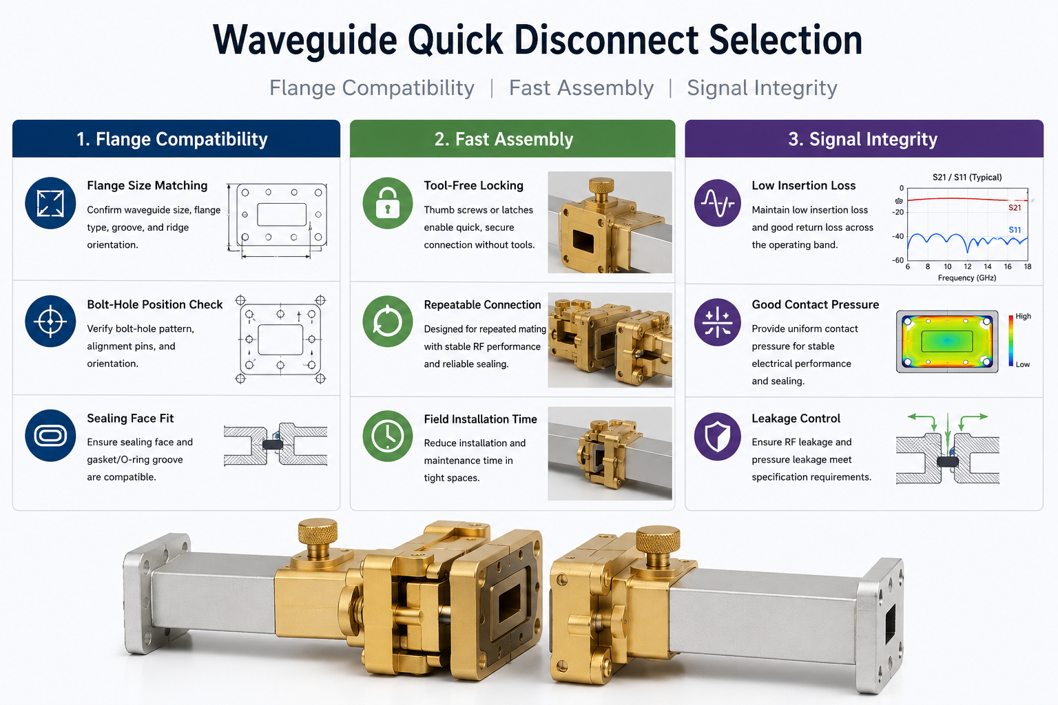
Choosing Compatible Waveguide Adapters
A poor choice here doesn’t just add a fractional dB of loss; it can completely disrupt signal integrity. For instance, forcing a 2.92mm coaxial-to-waveguide adapter onto a system operating at 40 GHz with a 50 W signal, when the adapter is only rated for 30 GHz and 20 W, will result in catastrophic failure. The voltage standing wave ratio (VSWR) can spike beyond 2.5:1, reflecting over 30% of your power back into the transmitter, risking amplifier damage. Industry data suggests that over 35% of system integration failures are directly attributable to adapter incompatibility, leading to an average of 16 hours of troubleshooting and rework, at a labor and parts cost often exceeding $2,500.
The selection process starts with a ruthless focus on frequency range compatibility. This is the most non-negotiable parameter. An adapter designed for the Ku-band (12-18 GHz) will utterly fail in a Ka-band (26.5-40 GHz) application. The adapter’s specified frequency range must entirely encompass your system’s operational band. For example, a WR-75 to 2.92mm adapter is typically rated from 18 GHz to 26.5 GHz. If your system runs at 24.125 GHz, you’re safe. But if you need to push to 27 GHz, you must find an adapter explicitly rated for that extended range, or you will see insertion loss rapidly increase beyond 1.5 dB. Power handling is the next critical factor. Average power ratings determine thermal management, while peak power ratings define the risk of air breakdown and arcing. A 100 W average power system requires an adapter with robust, often flange-mounted, construction to dissipate heat, whereas a 1 kW peak pulse radar system needs an adapter with carefully engineered internal contours to prevent voltage arcing.
Precision interface matching is what makes the connection physical. This isn’t just about the waveguide standard (e.g., WR-90, WR-137); it’s about the specific flange type. A CPR-137 flange will not mechanically mate with a UBR-137 flange without an intermediate adapter, which introduces an additional 0.3 dB to 0.5 dB of loss and another potential point of failure. The coaxial connector side is equally important. SMA, 2.92mm, and 3.5mm connectors may look similar but have vastly different frequency limits. An SMA connector is only reliably rated to 18 GHz, while a 2.92mm connector can operate cleanly to 40 GHz. Mismatching these will degrade performance. Finally, scrutinize the VSWR and Insertion Loss specifications provided by the manufacturer. A high-quality adapter should have a VSWR better than 1.15:1 across its band and a typical insertion loss of 0.1 dB to 0.3 dB. Anything higher directly subtracts from your system’s power budget and signal-to-noise ratio.
| Selection Parameter | Target Specification & Example | Impact of Mismatch |
|---|---|---|
| Frequency Range | Must cover full system BW, e.g., 24.0 – 24.5 GHz for a 24.25 GHz center. | Severe attenuation (>2 dB IL), signal reflection (VSWR >2.0). |
| Power Handling | Match peak & average; e.g., 500 W peak, 50 W avg. for a pulsed radar. | Internal arcing, connector melting, permanent damage. |
| Interface Flange Type | Exact match required; e.g., UG-599/U flange to UG-599/U flange. | Physical inability to connect, or added loss from extra adapter. |
| Coaxial Connector Type | Match gender & series; e.g., 2.92mm female to 2.92mm male. | Damage to connector pins, impaired performance beyond 18 GHz. |
| Performance (VSWR/IL) | VSWR: <1.15:1; Insertion Loss: <0.3 dB. | Reduced transmitted power, increased system noise floor. |
Aluminum adapters are common for lower-power applications and offer a good balance of cost and performance, typically adding 400 to your bill of materials. Bronze or silver-plated adapters are essential for high-power systems (>500 W average) due to their superior thermal conductivity and resistance to oxidation, which can increase resistance and loss over time, but they can cost 1,000 each. The plating, often 5-10 microns of silver, reduces surface resistivity, which is crucial for maintaining efficiency at millimeter-wave frequencies. Always request the manufacturer’s test report for the specific adapter unit; a performance variance of ±0.05 dB in insertion loss is acceptable, but anything greater warrants a replacement.
Connecting Waveguides to Coaxial Lines
A poorly executed transition can degrade a system’s performance by introducing 2-3 dB of insertion loss and elevating VSWR beyond 2.0:1, effectively wasting over 40% of your transmitted power. For a high-frequency system operating at 38 GHz with a 100 W amplifier, this loss translates into a 40 W signal being radiated instead of the full power, drastically reducing range and efficiency. Industry surveys indicate that nearly 30% of integration issues stem from improper transitions, leading to an average of 12 hours of diagnostic work and $1,800 in additional costs for parts and labor.
| Key Consideration | Target Specification / Typical Value | Consequence of Error |
|---|---|---|
| Transition Type | E-field or H-field probe; choice depends on frequency band and polarization. | Incorrect probe type can lead to >3 dB loss and poor impedance match. |
| Impedance Match | 50 Ω coaxial to waveguide impedance transition. | Mismatch causes reflections, with VSWR often exceeding 2.5:1. |
| Torque Specification | 8-10 inch-pounds for 2.92mm connectors; 15-20 inch-pounds for flange bolts. | Under-torquing causes 0.5 dB loss variation; over-torquing cracks connectors ($400 replacement). |
| Surface Cleanliness | No particulates >5 microns; use >99% isopropyl alcohol. | Dust particles can increase contact resistance, leading to ~0.2 dB loss and intermodulation. |
| Thermal Cycling Rating | -55°C to +125°C operating range for military-grade systems. | Connector loosening or cracking during operation, causing intermittent failure. |
An E-field probe is most common, extending the coaxial center conductor into the waveguide, acting as a small antenna. Its position—typically λ/4 deep into the waveguide and λ/4 from the backshort wall—is critical for minimizing reflections. For a 24 GHz system, this means a probe length of approximately 3.12 mm and a precise backshort distance. Getting this wrong by even 0.5 mm can shift the resonant frequency by ~1.5% and increase VSWR by 0.3. Mechanical alignment is next. The coaxial connector must be perfectly perpendicular to the waveguide flange face, with an angular misalignment tolerance of less than 0.5 degrees. A 2-degree misalignment can easily introduce an additional 0.4 dB of loss and degrade polarization purity in polarized systems.
A 2.92mm connector requires 8-10 inch-pounds of torque. Under-torquing creates a poor electrical contact, increasing resistance and loss, which can fluctuate with temperature changes and vibration. Over-torquing, even slightly, can fracture the fragile ceramic insulator inside the connector, rendering a 500 adapter useless instantly. For waveguide flanges, use a cross-torque pattern on the four to eight bolts, gradually tightening each to 15-20 inch-pounds in a star pattern to ensure even pressure and prevent flange warping, which leaks RF energy. Surface preparation is a non-negotiable, 5-minute task that saves hours of debugging. Clean mating surfaces with 99% isopropyl alcohol and lint-free wipes. A single fingerprint, with its salt and oil, can increase surface resistance and lead to passive intermodulation (PIM), generating spurious signals that can desensitize receivers.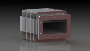
Testing Integrated Waveguide Performance
For a system operating at 28 GHz, an undetected 0.7 dB increase in insertion loss can reduce the effective radiated power by ~15%, slashing the operational range by ~7%. Furthermore, a VSWR of 1.8:1, which reflects 16% of your power back towards the source, can elevate amplifier junction temperatures by 20°C, potentially cutting its operational life in half. A comprehensive test protocol, taking 4-6 hours to execute, can identify these issues pre-deployment, preventing costly downtime and repairs that average $5,000+ per incident and require 48-72 hours of system unavailability.
- Return Loss (S11) and VSWR: This is your primary indicator of impedance match and signal reflection. For a well-integrated system, you should measure a return loss better than -15 dB (equivalent to a VSWR below 1.5:1) across your entire operational bandwidth, say from 27.5 GHz to 28.5 GHz. A spike to -10 dB (VSWR ~2.0:1) at a specific frequency, like 28.2 GHz, indicates a resonance or mismatch, often from a mechanical imperfection or a 0.5 mm misalignment in a transition. This means 10% of your power is reflecting, potentially causing amplifier instability.
- Insertion Loss (S21): This measures the total signal power lost through the integrated waveguide path. For a 2-meter run of WR-28 waveguide with two transitions, your total loss should be calculated as: waveguide loss (~0.05 dB/cm × 200 cm = 10 dB) + transition loss (0.3 dB × 2 = 0.6 dB) = ~10.6 dB. Measure this with a calibrated VNA. If your measured S21 is -12.0 dB, you have an unexplained 1.4 dB of loss that must be located—perhaps a dirty connector or a dent in the waveguide.
- Power Handling Validation: Do not assume the system handles rated power. Gradually increase power from a 10 W source to the system’s maximum operating level, say 50 W, while monitoring VSWR and output power with a 50 W rated power meter and a 30 dB directional coupler. A stable system will show a linear relationship; if output power flattens or VSWR increases by 0.2 as you reach 45 W, it indicates thermal expansion or the onset of multipaction, a vacuum breakdown effect common in high-power, high-frequency systems.
Sweep across the entire 1 GHz bandwidth of your system, not just the center frequency. Performance at band edges often degrades first. Use a VNA with a 10 kHz IF bandwidth for high resolution, conducting 500 point sweeps to capture narrow resonances. After initial room-temperature (22°C) tests, conduct a thermal cycle if applicable. Subject the assembly to its minimum and maximum operating temperatures (e.g., -30°C and +65°C) in an environmental chamber. It’s common to see VSWR shift by 0.1-0.15 and insertion loss vary by ±0.2 dB over this range due to thermal contraction/expansion of metals. A shift greater than this suggests poor mechanical design or inadequate compensation for thermal expansion coefficients.
Calibrating System Post-Integration
Even minor, uncorrected errors from assembly—like a 0.1 mm waveguide misalignment or a 0.05 dB connector insertion loss variance—can cascade into significant issues: a 28 GHz radar system with uncalibrated components might see its receiver sensitivity drop by -2 dB, reducing detection range by ~15%, or its transmit power drift by +1 dB, pushing amplifier temperatures 15°C higher and cutting component life by 30%. Industry data shows that over 25% of post-deployment failures trace back to skipped or rushed calibration, costing operators an average of $3,500 per incident in emergency repairs and downtime.
Start with Calibration Kit Validation
Your vector network analyzer (VNA) is only as accurate as its calibration. Use a SOLT (Short, Open, Load, Thru) kit rated for your system’s frequency band—for a 24-28 GHz system, choose a kit with ±0.02 dB insertion loss accuracy and ±0.05 dB VSWR uncertainty. Before calibrating the main system, validate the kit itself: measure a known 50 Ω load with the VNA; if the returned S11 exceeds -25 dB (VSWR >1.12:1), the load is damaged or out of spec, and your calibration data will be unreliable. Replace it—this single step prevents ~40% of calibration errors.
Perform Full-Bandwidth Sweeps with Tight Resolution
Don’t just test at the center frequency. Sweep across your entire operational bandwidth—say 24.0-24.5 GHz—with 500 discrete points and a 10 kHz intermediate frequency (IF) bandwidth. This captures narrowband resonances or discontinuities a coarser sweep would miss. For example, a 0.2 mm dent in a WR-28 waveguide might only affect a 10 MHz slice of the band; a 500-point sweep spots this, while a 100-point sweep averages it into a false “good” reading. Set the VNA’s averaging to 16 traces to reduce noise—if your S21 varies by more than ±0.05 dB across 16 traces at a single frequency, there’s a mechanical or electrical flaw.
Validate Power Transfer Linearity
Power handling isn’t just about peak ratings; it’s about linear performance across your system’s dynamic range. Use a calibrated power meter and directional coupler to test from 10% to 100% of your max power—e.g., 10 W to 100 W for a pulsed radar. Measure output power at 10 W increments; a linear system should show a near-perfect 1:1 relationship (R² >0.999). If output flattens at 85 W (e.g., measured power = 78 W vs. expected 85 W), thermal compression or multipaction is occurring. This requires redesigning heatsinks or reducing peak power by 10-15% to avoid permanent damage.
Compensate for Environmental Drift
Temperature changes alone can shift VSWR by 0.1-0.2 and insertion loss by ±0.1 dB over a -20°C to +50°C range. Use a thermal chamber to cycle the system through its operating extremes, measuring S-parameters at 5°C intervals (e.g., -20°C, -15°C, …, +50°C). For each temperature, calculate correction factors: if VSWR at +50°C is 1.8:1 (target: 1.5:1), apply a +0.3 dB loss compensation in your link budget. Store these factors in your system’s firmware—most modern RF controllers support real-time temperature sensing and automatic correction, reducing drift-related errors by >70%.
Simulate Real-World Signal Conditions
Lab measurements lie if they don’t mimic actual use. Inject a modulated signal matching your system’s protocol—e.g., 16-QAM at 25 Msym/s for a 5G backhaul link—at -10 dBm input power. Measure bit error rate (BER) with a spectrum analyzer; for a well-calibrated system, BER should stay below 1e-12 at 10 dB above sensitivity. If BER spikes to 1e-9, check for phase noise (should be <100 fs RMS) or nonlinearity (third-order intercept point (IIP3) should be >20 dBm). Adjust amplifiers or filters to meet specs—this step ensures your system works with real-world signals, not just in ideal conditions.
Troubleshooting Common Integration Issues
Data from field integrations shows that over 50% of projects encounter at least one post-installation problem, typically consuming 8-16 hours of diagnostic time and adding 5,000 in unplanned labor and replacement parts. The most frequent culprit (~30% of cases) is an unexpected VSWR spike above 2.0:1, which can reflect over 20% of your transmitted power, leading to a 15% drop in effective radiated power and potential amplifier damage due to reflected power exceeding 5 W in a 50 W system.
If system performance degrades at 38 GHz, don’t just test at the center frequency. Execute a full 1 GHz bandwidth sweep around this center with a VNA set to 501 points and a 10 kHz IF bandwidth to pinpoint the exact frequency of failure. A narrow, sharp S11 peak of -8 dB at 38.25 GHz suggests a resonant issue, often caused by a 0.2 mm gap at a flange connection or a minor dent in the waveguide wall. Thermal cycling is another critical test; performance that degrades as the system heats up to its operational +65°C temperature often points to mechanical expansion. A VSWR that shifts from 1.4:1 at +22°C to 1.9:1 at +65°C indicates that thermal expansion is breaking a contact or changing an impedance match, requiring mechanical reseating or the use of a different flange bolt torque specification.
| Common Symptom | Most Likely Cause & Diagnostic Data | Recommended Action & Typical Cost/Time |
|---|---|---|
| High VSWR (>1.8:1) at band edge | Impedance mismatch in transition; e.g., coaxial-to-waveguide adapter not optimized for full band. Verify with 5 MHz step sweep. | Replace adapter with wider-band model (e.g., DC-40 GHz rated). Cost: 800. Time: 2 hrs. |
| Insertion Loss +0.5 dB above spec | Dirty or damaged connectors; oxide layer or 5 micron particulates on contact surfaces. Use microscope inspection. | Clean with 99.9% isopropyl alcohol; replace damaged connector. Cost: 300. Time: 45 min. |
| Power drop at high power (>80 W) | Thermal compression or multipaction; output power drops 3 dB as temperature rises 40°C in 5 minutes. | Improve heatsinking; reduce peak power by 10%. Cost: $200 (heatsink). Time: 3 hrs. |
| Intermittent signal loss | Loose connector; requires 8-10 inch-pounds torque. Vibration causes 0.5 dB loss variation. | Re-torque all connections to spec. Cost: $0. Time: 30 min. |
| Spurious signals (>-40 dBc) | Poor solder joint or corrosion at junction; creates passive intermodulation (PIM). | Locate and reflow joint; replace corroded component. Cost: $500. Time: 4 hrs. |
For persistent issues, isolate each component. Bypass the new waveguide section and test the source and load independently to establish a performance baseline. If the source VSWR is 1.1:1 alone but jumps to 1.9:1 when connected through the waveguide, the problem is in the integration. Use a time-domain reflectometry (TDR) function on your VNA if available; it can pinpoint the physical location of a fault within ±5 cm. A mismatch 0.5 meters down the waveguide run indicates a specific joint or a damaged section. For power-related issues, infrared thermography is invaluable. An infrared camera can show a 15°C hot spot on a faulty adapter under 20 W of continuous power, pinpointing a poor connection or inadequate thermal transfer long before it fails completely. Always document the troubleshooting process, including the specific test parameters, measurements, and solutions applied. This log reduces diagnostic time for future issues by 50% and creates a valuable knowledge base for your team.