To measure waveguide antenna radiation patterns, use a vector network analyzer in an anechoic chamber: mount the antenna on a precision turntable, scan azimuth/elevation angles at 5° steps (2–40 GHz), capture S-parameters, and apply Fourier transforms to generate 3D pattern data, verifying gain and sidelobe levels.
Table of Contents
Set Up Test Equipment
For a standard X-band waveguide (8.2-12.4 GHz) test, your core gear includes a vector network analyzer (VNA) like a Keysight PNA or an Anritsu Shockline, a high-precision azimuth positioner (e.g., an Orbit/FR roll-azimuth turntable with 0.01° accuracy), a known-good reference horn antenna (say, a 20 dBi gain standard), and low-loss phase-stable coaxial cables (like 0.5″ diameter Andrew HELIAX with less than 0.5 dB loss per 10 meters at 10 GHz). Your test distance must meet the Fraunhofer far-field criterion, which for a typical 10 GHz antenna with a 15 cm aperture means you need at least 5 meters between your antenna under test (AUT) and the probe.
The first physical step is establishing a clear, unobstructed line-of-sight between the AUT and the probe antenna. This isn’t just about moving chairs out of the way; you need a dedicated, echo-free environment. An anechoic chamber is ideal, but if you’re in a large, empty lab, you must minimize reflections. Place RF-absorbent foam on large, flat surfaces like walls, floors, and ceilings within a 3-meter radius of the signal path. The height of both antennas should be set so their phase centers are aligned horizontally, typically around 1.5 meters off the ground. Before powering anything on, connect your setup mechanically: secure the AUT firmly to the positioner’s mast using its waveguide flange. Use a torque wrench to tighten the flange bolts to the manufacturer’s spec, usually 8 to 10 inch-pounds, to ensure a proper RF seal without warping the flange face.
Now, cable everything up. Run a low-loss cable from the VNA’s Port 1 directly to the input port of your AUT. The second cable goes from the VNA’s Port 2 to your probe antenna. Keep these cable runs as short as possible, absolutely under 6 meters each, to minimize signal loss. For a 5-meter test setup at 10 GHz, every extra decibel of cable loss reduces your dynamic range and increases measurement uncertainty. Before calibration, sweep the VNA in a standard S21 transmission measurement mode to check for any major impedance mismatches or unexpected loss; your system should show a baseline insertion loss that is stable and repeatable within ±0.2 dB when you gently move the cables. This confirms connectors are tight.
For a 10 GHz setup, this calibration is good for a bandwidth of about 2 GHz before drift becomes an issue. Your residual directivity after calibration should be better than 40 dB. Now, you are ready to position the antenna and start measuring.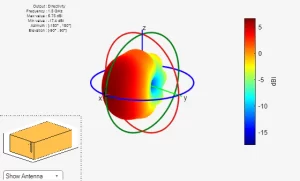
Position Antenna Correctly
For a standard gain horn operating at 10 GHz, a 0.5-degree tilt in the azimuth plane can introduce a measurable 0.8 dB error in peak gain and distort sidelobe levels by up to 3 dB. The goal is to ensure the Antenna Under Test’s (AUT) boresight is perfectly aligned with the central axis of your positioner and directly faces the probe antenna at your calibrated far-field distance, which for a 15 cm aperture antenna is typically 5.8 meters.
| Parameter | Target Value | Tolerance | Impact of Deviation |
|---|---|---|---|
| Boresight Alignment | 0° Azimuth, 0° Elevation | ±0.1° | >1 dB gain error; sidelobe asymmetry |
| Height Alignment | 1.5 m from ground | ±2 cm | Phase center misalignment |
| Polarization Tilt | 0° (Linear) | ±1.0° | >20 dB cross-pol contamination |
| Far-Field Distance | 5.8 m for 10 GHz, 15 cm aperture | ±10 cm | Near-field contamination in pattern nulls |
Place a high-accuracy digital level on the mounting flange of the positioner itself. Adjust the leveling feet until the readout shows less than 0.05 degrees of deviation in both the x and y axes. This ensures the axis of rotation is perfectly vertical. Next, mount the AUT onto the positioner’s mast. If your antenna has a waveguide flange, use a torque wrench to tighten the bolts to 10 inch-pounds in a star pattern to avoid warping the flange, which can distort the antenna’s aperture distribution. Now, the critical part: aligning the AUT’s theoretical boresight with the positioner’s rotational axis. This is a two-person job. One person slowly rotates the positioner 360 degrees while a second person observes the antenna’s outer casing from a fixed point several meters away, typically using a theodolite or a high-power laser alignment tool. The goal is to minimize the run-out, or the wobble, of the antenna’s outer edges as it spins. You want the maximum observed deviation to be under 0.5 millimeters at the antenna’s extremity, which for a 20 cm long horn translates to an angular error of less than 0.15 degrees.
Send a continuous wave (CW) signal from your VNA at the center frequency, say 10.3 GHz, at a low power level like 0 dBm. Configure the VNA to measure S21 in a real-time, max-hold mode. Now, command the positioner to sweep a narrow azimuth range, for example, from -5° to +5° with a step size of 0.1°. Watch the S21 trace. The peak power point on this trace is your electrical boresight. Note the exact azimuth angle where this maximum occurs, for instance, +0.3°. Now, using the positioner’s software, offset its zero position by this value. This electronically sets that peak point as your new 0° azimuth reference.
Measure Main Beam Direction
A misidentified peak by a mere 0.1 degree can propagate errors through every subsequent measurement, from gain calculation to sidelobe asymmetry. For a high-gain (e.g., 25 dBi) C-band radar antenna, this small angular error could translate to a pointing inaccuracy that misplaces a target by over 15 meters at a 10-kilometer range. The process involves a fine-resolution angular sweep around the estimated boresight to capture the exact angle of maximum radiation intensity with sub-degree precision, typically aiming for an accuracy of ±0.05° or better.
| Parameter | Target Value | Tolerance | Impact of Deviation |
|---|---|---|---|
| Azimuth Scan Range | ±10° from ref. | N/A | Must capture full main beam and first nulls |
| Angular Step Size | 0.1° to 0.25° | N/A | Determines precision of peak finding |
| Peak Finding Accuracy | 0.05° | ±0.02° | Directly impacts all gain and pointing specs |
| 3 dB Beamwidth | e.g., 4.5° | ±0.2° | Key metric for antenna resolution |
Set the VNA to a CW frequency at the center of your operating band, for instance, 10.0 GHz, with an output power of +10 dBm and an IF bandwidth of 100 Hz to maximize measurement sensitivity and minimize noise. Program the positioner to execute a highly precise azimuth scan. The scan range must be wide enough to fully capture the main lobe and just dip into the first nulls on either side; for a typical antenna with a 5.0-degree half-power beamwidth (HPBW), a ±10-degree sweep is a safe bet. The critical parameter here is the angular step size. Do not use a continuous rotation; you need discrete, stop-and-measure points. A step size of 0.1 degrees provides an excellent balance between data resolution and total measurement time, which for a 20-degree sweep will yield 200 individual data points.
As the positioner moves to each angle, the VNA records the transmitted power (S21 magnitude) in decibels (dB). The raw data will look like a sharp peak. Your job is to find the absolute maximum. Do not just rely on the highest recorded point from this coarse sweep. The true peak likely lies between two step points. Once you identify the two highest points from the initial data, perform a second, higher-resolution scan over a very narrow range, perhaps just ±0.3 degrees around the preliminary peak, using a finer step size of 0.02 degrees. This will give you 30 data points across a 0.6-degree span, allowing you to interpolate the true peak location with an accuracy of approximately ±0.01 degrees. The angle corresponding to the absolute maximum S21 value is your official main beam direction. Note this angle precisely; all future pattern cuts (e.g., E-plane, H-plane) will use this as their 0-degree reference.
Record Far-Field Data Points
A full spherical cut (0° to 360° in azimuth, -180° to +180° in elevation) with a 3-degree step resolution generates over 72,000 individual measurement points, a process that can take 6 to 8 hours to complete with a high-degree of accuracy. The goal is to capture not just the main beam but also sidelobes that may be -30 dB or more below the peak, requiring your system to have a noise floor at least 10 dB below that level.
For a principal plane cut (e.g., the E-plane), a typical scan ranges from -90 degrees to +90 degrees in elevation, with the azimuth fixed at the previously determined boresight angle of 0.0 degrees. The choice of angular step size is a direct trade-off between resolution and measurement time. For most engineering purposes, a step of 0.5 degrees to 1.0 degree is sufficient, creating a sweep of 180 to 360 points for this single cut. However, to resolve deep nulls and sharp sidelobes accurately, a finer step of 0.2 degrees is recommended, increasing the point count to 900 for the 180-degree sweep and extending the measurement duration to approximately 45 minutes per plane.
Set the IF bandwidth to 100 Hz for a good signal-to-noise ratio without excessive sweep time. At each stop, the positioner must settle completely for a period of 150 milliseconds to dampen any mechanical vibration before the VNA records the S21 magnitude in dB. This settling time is non-negotiable; without it, micro-vibrations can introduce ±0.15 dB of random error into each measurement. The system must record this value, along with the precise azimuth and elevation angles from the positioner’s encoder, with an angular accuracy of ±0.01°. For a complete characterization across multiple frequencies, you will repeat this entire process at specific points across the operational band, such as the lower band edge (8.2 GHz), center frequency (10.3 GHz), and upper band edge (12.4 GHz), tripling the total data acquisition time.
The temperature of the lab should remain stable within ±2°C, as thermal expansion can physically misalign your setup and alter cable phase length. Check the baseline noise floor every 30 minutes by commanding the positioner to a deep null point and ensuring the received power has not increased by more than 0.3 dB. This validates that no external interference or system degradation has occurred. The final output is a massive data set of angle-power-frequency triplets, typically a .csv file exceeding 5 MB in size, ready for processing and plotting.
Plot Radiation Pattern Graph
The standard is a polar plot on a logarithmic (dB) scale, typically spanning a 60 dB dynamic range from the peak, with angular axes from -180° to +180° or 0° to 360°. For a standard gain horn, this plot will clearly show a main beam with a -3 dB beamwidth of approximately 4.5 degrees and sidelobes suppressed by -20 to -25 dB. Plotting is not just visualization; it’s the first step in quantitative analysis, where a 0.5 dB error in the graph’s scale can lead to a significant misjudgment of antenna quality.
| Graph Parameter | Standard Value | Purpose & Notes |
|---|---|---|
| Dynamic Range | 60 dB (from peak) | Must be set to reveal lowest sidelobes and nulls. |
| Angular Range | ±90° or ±180° | Shows full pattern or focuses on main beam region. |
| Radial Scale (dB) | 10 dB per major ring | Standard division for easy reading of dB levels. |
| Reference Line | 0 dB = Peak Gain | All values are plotted relative to the main beam peak. |
| 3-dB Beamwidth | Measured in degrees | Directly read from plot at the -3 dB points. |
The first step is data preparation. Your raw data is a list of angles and corresponding relative power values in dB. Import this .csv file containing, for example, 360 points at 1-degree intervals into your plotting software (e.g., Python with Matplotlib, MATLAB, or Excel). Normalize your data by identifying the absolute maximum power value from your main beam direction and subtracting this value from every single data point. This sets your peak gain to 0 dB, and all other values become negative dB values relative to this peak. This normalization is crucial for comparing patterns and measuring relative parameters like sidelobe levels.
Now, create a polar plot. Set the angular axis (theta) to run from -180 degrees to +180 degrees. Set the radial axis to a logarithmic scale, which is represented in decibels. The critical setting here is the radial limit. Set the minimum radial value to -60 dB if your measurement system’s noise floor is at -65 dB, ensuring you capture the deepest nulls and lowest sidelobes without displaying excessive noise. The major grid rings should be set every 10 dB for clear visual reference. Plot your normalized data. The resulting line will show the main beam as a prominent spike, with smaller spikes (sidelobes) surrounding it and sharp dips (nulls) in between.
Analyze Gain and Sidelobes
For a communication system, a 1 dB error in gain calculation can reduce your effective range by approximately 12%, while a sidelobe that is 3 dB higher than specified can cause unacceptable co-channel interference. The goal is to extract numerical values with high precision, including peak gain in dBi, half-power beamwidth (HPBW), first sidelobe level (SLL), and front-to-back ratio, typically aiming for measurement accuracies within ±0.25 dB and ±0.1°.
The definitive performance summary for a standard X-band horn might read: Peak Gain: 19.8 dBi ±0.2 dBi, 3-dB Beamwidth: 4.5°, First Sidelobe Level: -24.5 dB, Front-to-Back Ratio: 35 dB.
You know the relative pattern from your normalized plot, where the peak is 0 dB. To find the absolute value in dBi, you must reference your system calibration using the gain substitution method. You measured a known reference antenna, say a 20.0 dBi standard gain horn, at the same 5.8-meter distance and 10.3 GHz frequency. Your VNA recorded an S21 value of -45.2 dB for this reference antenna. When you measured your Antenna Under Test (AUT), the peak S21 value was -44.0 dB. The absolute gain of your AUT is calculated as: G_AUT = G_ref + (S21_AUT – S21_ref) = 20.0 dBi + (-44.0 dB – (-45.2 dB)) = 20.0 dBi + 1.2 dB = 21.2 dBi. This +1.2 dB difference directly translates to the gain value, giving you a precise, calibrated result.
Next, analyze the sidelobe levels (SLL). Zoom into your plotted pattern data around the first major lobe outside the main beam, typically occurring between 15° and 25° off boresight. Use your software’s data cursor tool to find the absolute maximum value within this angular region. This point is the first sidelobe peak. Its value, read directly in dB relative to the main beam, is the SLL.
For a well-designed antenna, this should be -20 dB or lower; a value of -24.5 dB indicates excellent suppression. Repeat this process for the second and third sidelobes, which are often 2-3 dB lower than the first, providing a complete picture of the pattern’s roll-off. Immediately after the first sidelobe, identify the deepest null, which could reach -42 dB or lower. A shallow null, above -30 dB, often indicates measurement errors like reflections or poor alignment.