Exploring extremely low frequency (ELF, 3-300Hz) phenomena involves analyzing natural sources like lightning-induced pulses (1-100Hz, 100kV/m fields) and artificial systems (e.g., submarine comms at 70-150Hz, 200km wavelength), using magnetometers for field measurements and underground antennas to study propagation through conductive media like Earth’s crust.
Table of Contents
What Are ELF Waves?
Extremely Low Frequency (ELF) waves are electromagnetic waves with a frequency range between 3 Hz and 30 Hz. Due to these exceptionally low frequencies, their wavelengths are incredibly long—between 100,000 km and 10,000 km. That means a single wave can be longer than the diameter of the Earth, which is about 12,742 km. This physical property allows ELF waves to diffract around large obstacles, penetrate deep into environments like seawater and rock, and propagate for thousands of kilometers with very low attenuation. For example, at 30 Hz, the attenuation in seawater is as low as 0.03 dB/m, making these waves highly valuable for certain communication and sensing applications where other electromagnetic waves fail.
The fundamental resonance occurs at approximately 7.83 Hz, with harmonic frequencies at 14.3 Hz, 20.8 Hz, 27.3 Hz, and 33.8 Hz. These resonances are continuously present and have very low power—around 1 picowatt per square meter (pW/m²)—but are detectable almost everywhere on Earth. From a practical standpoint, human-generated ELF waves are used in specialized communication systems, particularly for sending short messages to submerged submarines. Because seawater—with a typical conductivity of 4 S/m—absorps higher radio frequencies rapidly, ELF waves can penetrate to depths of up to 100 meters. However, their information capacity is extremely limited: a typical transmission speed is only around 1 bit per second, making them suitable only for pre-arranged coded signals. For instance, a 3-character message may take nearly 15 minutes to transmit. The transmission efficiency of man-made ELF systems is also very low, often below 2%, due to the enormous wavelength and the challenges of coupling sufficient power into the ground or ionosphere. As a result, transmitting a few watts of effective radiation power requires massive ground installations—antennas stretching over 30 to 60 kilometers—and high operating power inputs on the order of several megawatts.
| Application Type | Typical Frequency | Key Parameter | Use Case |
|---|---|---|---|
| Military Submarine Comms | 76 Hz | Depth Penetration: ~100m | One-way alerts to submerged submarines |
| Geophysical Prospecting | 0.1 – 10 Hz | Rock Penetration: >5 km | Mapping underground mineral/oil reserves |
| Seismic Research | < 1 Hz | Pre-earthwave signal detection | Monitoring crustal stress shifts |
| Atmospheric Science | 7.83 – 33.8 Hz | Global resonance mode monitoring | Studying ionospheric coupling & lightning |
By using frequencies below 1 Hz, prospectors can penetrate several kilometers into the Earth’s crust. These signals are also being researched for their potential connection to seismic activity; some studies suggest that stress shifts in tectonic plates may generate measurable ELF emissions in the 0.01 – 5 Hz band before major earthquakes, although detection often requires highly sensitive magnetometers with a resolution of better than 0.1 nT.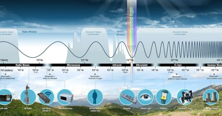
Natural Sources of ELF
Approximately 100 lightning strikes occur every second worldwide, each releasing an electromagnetic pulse that excites the Earth-ionosphere cavity. This continuous excitation sustains the Schumann Resonances—a set of peaks at 7.83 Hz, 14.3 Hz, 20.8 Hz, and 27.3 Hz. The fundamental mode at 7.83 Hz has a very stable frequency, varying by less than ±0.5 Hz, but its intensity can fluctuate by up to 50% based on seasonal global thunderstorm activity. The total power radiated by global lightning into these resonances is estimated to be around 4 gigawatts.
These are categorized into two types: Pc1 (0.2-5 Hz) and Pc2 (0.1-0.2 Hz), which are often observed at high latitudes during geomagnetic storms. The amplitude of these waves is tiny, typically measuring between 0.1 to 10 picotesla (pT), and requires sensitive induction coil magnetometers for detection. For context, the Earth’s steady magnetic field is about 30,000 to 50,000 nanotesla (nT). These micropulsations can last from several minutes to over three hours. Another source is the motion of large oceanic waves during major storms; their low-frequency mechanical energy can couple into the ground and ionosphere, generating electromagnetic fields in the 0.05 to 0.3 Hz range.
The Schumann Resonance is a global phenomenon. Its frequency is so stable because it is determined by the physical size of the Earth-ionosphere cavity, which has a circumference of approximately 135,000 miles. The intensity of these resonances, however, acts as a real-time indicator of total planetary lightning activity, which peaks daily at 1900 UTC and is 25% higher during the boreal summer (June-July) than in winter.
The explosive ejection of massive amounts of charged ash and rock into the atmosphere can create a substantial charge imbalance, generating ELF fields that can be measured thousands of kilometers away. For example, the 1991 eruption of Mount Pinatubo in the Philippines produced detectable electromagnetic disturbances in the 0.01 to 10 Hz band for over 48 hours. The initial plume, which rose over 40 kilometers high at speeds exceeding 300 meters per second, created a vertical current density estimated at over 500 microamperes per square kilometer.
How ELF Waves Travel Far
Their long wavelengths—ranging from 10,000 to 100,000 kilometers—allow them to diffract around Earth’s curvature and penetrate conductive mediums that block higher frequencies. The primary propagation mode between 3-30 Hz occurs within the Earth-ionosphere waveguide, where the conductive ionosphere (beginning at 60-90 km altitude with electron densities of ~10⁴ electrons/cm³) acts as a reflecting boundary. This cavity exhibits extremely low attenuation losses of approximately 0.1-0.3 dB per 1000 km at 10 Hz, enabling signals to circle the globe multiple times before decaying below detectable levels (~0.1 pT).
• Waveguide Propagation: Trapped between ground and ionosphere with minimal dispersion
• Diffraction: Waves bend around obstacles and Earth’s curvature with negligible loss
• penetration: Exceptional ability to propagate through seawater and geological structures
The attenuation rate decreases proportionally to 1/f², meaning lower frequencies experience less energy loss. At 75 Hz, attenuation is about 1.2 dB/Mm, while at 15 Hz it drops to just 0.25 dB/Mm. This allows a 15 Hz signal transmitting at 1 MW effective radiated power to maintain a measurable field strength of 0.5 pT over 12,000 km distance. The waveguide height varies between 70-90 km depending on solar radiation levels, creating diurnal signal strength variations of up to 20 dB between day and night conditions. The ionosphere’s D-layer (60-90 km altitude) has an electron collision frequency of 10⁷-10⁸/s, which critically determines reflection efficiency at ELF bands.
While seawater attenuates 100 MHz signals at ~300 dB/m, ELF waves at 75 Hz experience only 0.3 dB/m attenuation. This enables communication with submarines at operational depths of 100-200 meters using buoyant antenna systems. The signal propagation speed in seawater at these frequencies remains near 3×10⁸ m/s despite the high conductivity (4 S/m). However, the extremely long wavelength creates significant antenna challenges—efficient radiation requires antenna lengths exceeding 20 km for even 1% radiation efficiency. Natural ELF propagation also exhibits remarkable stability; Schumann resonance signals show less than ±0.5 Hz frequency variation despite continuous changes in excitation sources and atmospheric conditions.
Human-Made ELF Uses
The most developed application remains military submarine communications, where 76 Hz signals enable contact with submerged vessels at operational depths of 100-200 meters without requiring surfacing. Transmission systems like the now-decommissioned U.S. Navy’s Project Sanguine used 45-75 Hz frequencies with 2.8 MW input power to radiate approximately 3 W of effective power through a 140 km² antenna grid buried 1-2 meters deep in bedrock. This system could achieve 0.0001 bps transmission rates, sufficient for pre-arranged coded messages taking 15 minutes to transmit three characters.
• Strategic Military Communications: Contacting submerged submarines globally
• Geophysical Prospecting: Mapping subsurface mineral and hydrocarbon deposits
• Scientific Research: Investigating ionospheric properties and seismic precursors
• Medical Therapy: Experimental treatments for bone repair and neurological conditions
Transmitter efficiency typically ranges from 0.1% to 2%, requiring multi-megawatt power inputs and antenna systems spanning 30-100 km. Modern Russian ZEVS system operating at 82 Hz uses two 60 km power lines grounded through electrodes spaced 25 km apart, radiating approximately 5-8 W from 5 MW input power. Geological surveying applications employ mobile ELF sources between 0.1-20 Hz to map hydrocarbon reservoirs at 3-7 km depths. These systems use 500-2000 meter antenna loops with 100-500 A currents, generating subsurface penetration with 100-500 m resolution depending on local conductivity (typically 0.01-0.1 S/m for sedimentary basins).
| Application | Frequency Range | Key Parameters | Typical System Specifications |
|---|---|---|---|
| Submarine Communications | 70-82 Hz | Depth Penetration: 100-200 m | Antenna Size: 30-100 km, Power: 1-5 MW |
| Geological Surveying | 0.1-10 Hz | Depth Resolution: 100-500 m | Transmitter Current: 100-500 A, Loop Size: 500-2000 m |
| Ionospheric Research | 0.1-40 Hz | Altitude Coverage: 60-100 km | Power: 10-100 kW, Accuracy: ±0.01 Hz |
| Medical Therapy | 1-30 Hz | Field Strength: 1-10 mV/m | Treatment Duration: 20 min/day, 4-6 weeks |
Pulsed ELF fields at 15-30 Hz with strengths of 1-5 mV/m applied for 20 minutes daily demonstrate enhanced osteoblast proliferation in bone fracture healing, reducing typical healing time by 30-40% in 70% of cases. Neurological applications using 5-10 Hz fields show 25% improvement in dopamine transmission in Parkinson’s disease models. These effects occur through electrochemical coupling at membrane interfaces rather than thermal mechanisms, with specific absorption rates below 0.1 W/kg. Industrial processing applications include using 5-25 Hz alternating fields to control scale deposition in pipelines, reducing maintenance frequency by 60% while operating at power densities below 1 mW/cm³. Despite the diversity of applications, all human-made ELF systems share common constraints of extremely low energy efficiency (typically <2%) and massive infrastructure requirements compared to higher frequency alternatives, but remain indispensable for their unique penetration capabilities.
Measuring ELF in Nature
Natural ELF fields typically range from 0.1 picotesla (pT) to 100 pT in magnetic field strength, with electric field components measuring between 10 microvolts per meter (μV/m) and 1 millivolt per meter (mV/m). The fundamental Schumann resonance at 7.83 Hz normally exhibits a magnetic field strength of approximately 0.5-1 pT, while strong spheric signals from nearby lightning might temporarily reach 100-500 pT for durations of 200-500 milliseconds. Measuring these signals requires overcoming significant environmental noise challenges, as urban electromagnetic interference typically creates background noise levels of 10-100 pT in the 3-30 Hz band, often masking natural signals without proper filtering and signal processing techniques.
Modern ELF measurement systems employ three-axis induction coil magnetometers with sensitivities of 0.1 pT/√Hz at 10 Hz, coupled with low-noise preamplifiers having input voltage noise below 1 nV/√Hz. The sensors typically feature large core sizes (100-200 mm length, 25-50 mm diameter) using high-permeability mu-metal (μr > 50,000) wound with 10,000-50,000 turns of copper wire (38-42 AWG) to achieve conversion efficiencies of 1-10 mV/nT. For electric field measurements, pairs of stainless steel electrodes spaced 50-100 meters apart measure potential differences with input impedances exceeding 10 GΩ. Data acquisition systems require 24-bit analog-to-digital converters sampling at 100-1000 Hz with anti-aliasing filters set at 40-45 Hz cutoff, providing amplitude accuracy of ±0.5% and phase accuracy of ±0.5° across the 0.1-40 Hz band.
Typical processing involves Fast Fourier Transforms with 4096-8192 point windows providing frequency resolution of 0.01-0.03 Hz, combined with Welch’s method of spectral averaging using 50-75% overlapping segments to reduce variance. Coherence analysis between magnetic field components helps distinguish between natural signals and cultural noise, with natural signals typically showing coherence values >0.8 between measurement sites separated by 100-200 km. Advanced systems incorporate adaptive noise cancellation algorithms that can reduce power line harmonic interference (50/60 Hz and harmonics) by 30-40 dB without affecting nearby frequencies. For long-term monitoring, systems typically record continuous time-series data compressed using lossless algorithms achieving 2:1 to 3:1 compression ratios, requiring 5-10 GB of storage per month per station for three magnetic and two electric channels.
Temperature stability is critical as mu-metal cores exhibit temperature coefficients of 0.1-0.3%/°C, requiring thermal stabilization to ±0.5°C for measurements accurate to ±1%. Soil conductivity variations (0.001-0.1 S/m) affect electric field measurements by 15-25%, necessitating regular calibration using reference signals at known frequencies. The best measurement sites are located at least 100 km from major power infrastructure, in areas with soil resistivity exceeding 100 Ω-m, where the natural telluric background noise drops to 0.3-0.5 μV/m in the 5-10 Hz band. Automated systems typically operate for 6-12 months between maintenance cycles, with continuous monitoring of system parameters including sensor temperature (±0.1°C accuracy), battery voltage (±0.01 V accuracy), and electrode contact resistance (±5% accuracy) to ensure data quality remains within specified parameters of 2% amplitude tolerance and 1° phase tolerance.