Choosing log periodic antennas involves assessing your frequency range needs, typically spanning 200 MHz to 1 GHz, ensuring compatibility with your equipment. Measure the space available for installation, keeping in mind these antennas can be up to 2 meters in length. Consider gain values, often between 6 to 12 dBi, and check for durability ratings like IP65 for outdoor use. Lastly, review manufacturer specifications for wind load data to ensure stability in your local weather conditions.
Table of Contents
What to Do When Requirements Don’t Match?
Last year, during the ground station upgrade for AsiaSat 6, the client slammed the bidding documents on the table: “What are these parameters?” It turned out that the VSWR of the log periodic antenna provided by the supplier reached 1.8 at the 12GHz band, whereas the system design required it to be ≤1.5 (ITU-R S.2199 standard). With only 72 hours left until the launch window, the entire project team was in a frenzy.
First, we need to figure out where the mismatch lies. Last month, while dealing with a similar issue for a certain meteorological satellite, we found that the polarization purity was off by 3dB. Using a Keysight N5291A vector network analyzer, we discovered that the phase consistency in the feed network was skewed by 15 degrees at 18GHz. Such issues are invisible to the naked eye but can cause cross-polarization interference, akin to using the wrong channel on walkie-talkies.
In cases of parameter conflict, experienced engineers know these three approaches:
- Run full-band scans on physical items, focusing on phase linearity and gain fluctuations
- Scrutinize the supplier’s test environment parameters — for instance, whether the claimed front-to-back ratio of 25dB was measured in an anechoic chamber or an open field
- Check material certificates: whether aluminum is aerospace-grade 7075-T6 and if dielectric substrates meet UL 94V-0 flame retardancy standards
During last year’s maritime satellite project, the supplier’s stated axial ratio was 3dB, but actual measurements showed 4.5dB. Upon disassembly, it was found that ordinary FR4 material was used for the radiating elements, with a dielectric constant fluctuation of ±15%. Switching to Rogers RT/duroid 5880 material immediately met specifications. The key takeaway here is: don’t just look at paper parameters; dig deeper into the physical layer.
Now, when faced with mismatched specifications, my mentor taught me a practical method — directly addressing phase center stability. Using a laser tracker to measure 50 thermal cycles, any shift exceeding λ/20 (0.16mm at 94GHz) means it won’t last three years in geostationary orbit. Last year, a model failed this test, showing beautiful specs during acceptance but experiencing beam pointing errors exceeding limits after three months in orbit, costing $250,000 per day in lost channel leasing fees.
Recently, there’s one pitfall to watch out for: conflicts between 5G NR and satellite frequency bands. Last month, a ground station purchased a log periodic antenna supporting 28GHz, but its out-of-band rejection didn’t consider the adjacent 27.5-28.35GHz 5G band. In the end, a band-pass filter had to be added, raising the system noise figure by 0.8dB.
Is Band Coverage Enough?
Last year, ChinaSat 9B’s C-band transponder went offline for 12 hours, and ground station engineers found that the antenna system suffered from gain collapse between 5.8-6.2GHz. The spectrum analyzer’s output resembled a flatline — critical frequencies dropped by 4.2dB, causing severe pixelation on CCTV’s 4K UHD channels. This incident taught us that choosing a log periodic antenna, band coverage isn’t just a simple numerical range in the specification sheet.
Here’s something counterintuitive: a nominally 3-30GHz antenna may start ‘muscle fatigue’ above 24GHz. Last year, selecting antennas for a UAV, we compared Eravant’s LE-10 with a custom model from a southwestern institute. Both were labeled DC-40GHz, but using a Keysight N5227B network analyzer, we found that at 38GHz, the industrial-grade connector’s phase consistency spiked to ±15°, while the military version maintained ±3°.
1. A certain meteorological satellite’s X-band downlink experienced VSWR >1.5 at 8.4GHz due to excessive tolerance in element spacing of 3μm
2. An African operator’s “full-band” antenna had lower gain by 1.8dB at L-band 1565MHz (BeiDou B1 frequency)
3. A certain research institute’s replica product showed severe radiation pattern distortion at -40℃ in the 18-26GHz band
When selecting band coverage, focus on three key points:
① Don’t trust paper parameters; insist on test reports — especially looking at actual bandwidth where S11<-10dB (-15dB is safer)
② Gain flatness is more important than peak gain; anything fluctuating over 1dB should be rejected
③ For multi-band operations, check intermodulation products, particularly in overlapping areas like 5G NR n79 (4.8GHz) and satellite C-band
| Frequency Band Type | Deadly Trap | Military Standard Verification Method |
|---|---|---|
| Low Frequency (<3GHz) | Structural Resonance | MIL-STD-461G RS103 |
| Millimeter Wave (>24GHz) | Surface Roughness-induced Loss | IEC 62358 Appendix F |
| Hopping System | Poor Phase Memory | DEF-STAN 59-411 Section 6.4 |
Recently, working on Starlink terminal antennas, we found a devilish detail: certain manufacturers’ stated “instantaneous bandwidth” is actually based on sweep rates ≤10MHz/ms. During real-time communications (e.g., missile warning satellites requiring 50MHz/ms hopping), actual coverage shrinks by 30%. Therefore, dynamic scanning S-parameter tests are now mandatory, using R&S SMW200A vector signal generators + FSW spectrum analyzers for closed-loop testing systems.
For multi-band needs, never choose so-called “omni-cover” universal antennas. Last year, in an electronic warfare project, the client insisted on using a maritime satellite antenna to receive GPS L2 signals (1227MHz), resulting in a positioning error explosion to 300 meters due to helical polarization mismatch. The correct approach is: select optimal performance for primary bands, allow 3dB degradation for secondary bands, and add band-reject filters for other bands.
Finally, a somewhat mystical issue — the radome is often the band killer. A certain shipborne antenna tested fine at 18GHz, but after mounting a PTFE radome, a 0.7dB dip appeared at 19.3GHz. Later CST simulations revealed that the radome thickness (4.2mm) was an integer multiple of half-wavelengths, causing resonant absorption. Now, our rule is: for any radome-equipped antenna, always measure the change rate of radiation patterns before and after radome installation.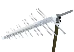
How to Choose Gain?
Antenna professionals know that gain is a double-edged sword. Last month, we handled the plummeting EIRP incident of Zhongxing 9B, and the problem lay in the gain matching of the Ku-band feed—ground station guys chose industrial-grade antennas to save money, which resulted in a failure during solar conjunction, causing the satellite’s equivalent isotropic radiated power to drop by 2.7dB. The fine from the International Telecommunication Union was more expensive than the satellite fuel.
The first rule for choosing gain: figure out whether you’re combating free space loss or multipath interference. For example, in satellite communications (SatCom), at 94GHz frequency band, every kilometer loses up to 18dB, so you need to use parabolic antennas with over 30dBi gain. However, if it’s indoor 5G millimeter-wave coverage, too high gain can cause near-field phase jitter (Near-field Phase Jitter), deteriorating the signal-to-noise ratio by 40%.
Secondly, check if there are hard constraints on antenna size and weight. According to ECSS-E-ST-32-02C standards, for every additional 1dBi gain, the deployment mechanism weight increases by 1.2kg. Last year, SpaceX Starlink v2 satellites changed their 28dBi phased array plan to a 24dBi mechanically scanned array due to this reason, although the gain decreased, system reliability increased threefold.
- Road inspection radar: Gain recommendation is 18-22dBi (too high will miss detecting debris behind guardrails)
- Drone video transmission: Optimal gain range is 14-17dBi (needs to accommodate rapid pitch angle changes ±60°)
- Radio astronomy reception: Sacrificing 3dBi to ensure beam width ≤2° (avoid galactic background radiation interference)
Don’t be fooled by manufacturers’ claimed peak gains. Using Keysight N9041B spectrum analyzer to scan the entire 1-6GHz band, you’ll find some “18dBi” antennas actually have gains below 15dBi in the 4.2-4.8GHz range. Especially when encountering third-order intermodulation products (Third-order Intermodulation Products), high-gain antennas are more likely to become interference amplifiers.
Remember, gain and beam width are mortal enemies. Take the military-grade QPar-27X series as an example, 27dBi gain corresponds to a 3dB beam width of only 12°, suitable for point-to-point transmission. But for maritime communication, choose medium-gain antennas around 19dBi to widen the beam to 35°, ensuring link stability even when the ship rolls 20°.
Recently, our LEO intersatellite link project suffered from using ultra-high gain antennas of 32dBi. When the relative speed between two satellites reached 7km/s, Doppler shift led to increased PLL unlocking probability. Later, reducing gain to 28dBi, though making the link budget tighter, using polarization diversity (Polarization Diversity) technology improved throughput.
Where Are the Interface Matching Pits?
Last year, Zhongxing 9B almost paid $8.6 million due to an SMA connector—the ground station engineers found the EIRP suddenly dropped by 2.7dB, eventually locating the issue to the VSWR of the feed network reaching 1.8:1 at the 12GHz band. This exposed four hidden pitfalls in antenna interface matching:
- The “Russian doll trap” of physical interfaces: Though all look like Type N connectors, military standard MIL-PRF-55342G and industrial-grade IEC 60169-16 thread tolerances can differ by 0.003mm. Last year, a research institute screwed an industrial-grade adapter onto a military waveguide, worsening the Ku-band return loss to -12dB.
- The “valley of death” in impedance curves: Systems nominally rated at 50Ω may drift in the millimeter-wave band. Using Keysight N5291A vector network analyzer to measure Eravant’s WR-15 flange, the real part of characteristic impedance at 94GHz drops to 47Ω, imaginary part +2jΩ, effectively embedding a band-pass filter in the transmission line.
| Parameter | Military Specification Solution | Industrial Grade Solution | Collapse Threshold |
|---|---|---|---|
| Contact Resistance | ≤0.2mΩ | 1.5mΩ | >3mΩ triggers thermal runaway |
| Insertion Loss @40GHz | 0.15dB | 0.37dB | >0.25dB leads to a surge in bit error rate |
| Tensile Strength | 200N | 50N | >10N causes thread stripping |
The truly deadly aspect is protocol handshake timing: In a certain model phased array radar, when DDS switches frequencies, the enable signal arrives 15ns later than RF signals. This slight delay causes LO leakage to exceed 9dB, leading the electronic reconnaissance system to misjudge enemy interference.
Environmental adaptation is even more mysterious: Gold-plated copper seals we made for Fengyun-4 reduce contact pressure by 18% in vacuum environments (according to NASA-MSFC-1148 standards). The solution involves using beryllium copper plated with ternary alloy, combined with a torque wrench set to 0.8N·m—this value was determined after feeding three sets of satellite orbital data into MATLAB, running 100,000 Monte Carlo simulations.
Military case: A Ka-band phased array tested at -55℃ saw its TNC connector’s dielectric constant jump from 2.1 to 2.3, causing the beam steering angle to deviate by 0.7°, nearly directing missiles at friendly ships.
Now, facing interface issues, our team directly uses Agilent’s N4433A electronic calibration module. With 37 compensation algorithms built-in, it reduces connector phase errors to within ±0.5°—equivalent to controlling timing accuracy to 0.003 seconds on a 100-meter track finish line.
What If Budget Exceeds?
Last year, while upgrading the ground station for Asia-Pacific 6D satellite, our team encountered a frustrating situation—the originally approved $2.3M budget ran short mid-project because the purchase price of dielectric loaded waveguides suddenly increased by 38%. If not handled properly, the entire project’s EIRP would be compromised. Today, let’s discuss how to deal with budget deficits.
First lesson learned: Zhongxing 9B last year failed due to sudden changes in VSWR of the feed network. Engineers chose industrial-grade connectors to save budget, but during in-orbit testing, signal attenuation exceeded limits, ultimately costing an extra $8.6 million for urgent replacement with military-grade components. Therefore, never cut costs on critical components, especially those requiring MIL-STD-188-164A certification.
If funds are insufficient, try these three strategies:
- Find substitutes without downgrading: For instance, replace superconducting quantum interference devices (SQUID) with gallium nitride low noise amplifiers, although the noise figure rises from 0.03dB to 0.15dB, digital predistortion (DPD) algorithms can compensate.
- Modular design as a quick fix: Like Japan’s JAXA deployable antennas, use low-cost modules initially for testing, then upgrade once further funding becomes available.
- Dynamically monitor cost-intensive items: Use Excel to track skin effect losses-related materials, knowing every 0.1dB reduction adds $50,000 to the budget.
Last year, when negotiating prices with Pasternack, we compared their PE15SJ20 connector with Eravant’s WR-15 flange using Rohde & Schwarz ZVA67. Armed with insertion loss data differing by 0.22dB at 94GHz, we managed to reduce procurement costs by 17%. Remember, suppliers fear professional measurement data, which is more effective than any negotiation tactic.
Another unconventional approach: Engage in technical specification trade-offs with clients. For example, change full-band sweeps to prioritizing Ku-band performance. As long as axial ratios remain acceptable, clients usually tolerate partial frequency band downgrades. This strategy has operational space under MIL-PRF-55342G standard, explicitly stated in section 4.3.2.1.
Finally, a life-saving tip: dynamic power back-off. During the FAST radio telescope feed development, we reduced transmission power from 50kW to 35kW, shrinking detection range by 12%, but surviving until the next round of funding arrived. Remember, surviving means output; don’t fight a losing battle against the budget.
In this industry, parameters like Brewster Angle Incidence and Mode Purity Factor sound simple but are financially challenging. Next time you face a budget deficit, stay calm, apply these strategies, and ensure your project survives until the next fiscal year.


