Choose a coaxial cavity filter when lower-frequency operation, compact packaging, and direct 50 Ω connections are the main constraints. Favor waveguide at microwave and millimeter-wave frequencies when low loss, power handling, or existing waveguide ports justify it. There is no universal GHz or watt threshold. Compare both designs at the same bandwidth and rejection requirements, then include adapters in the loss and power budget.
The examples below cover conventional metal hollow-waveguide and coaxial cavity bandpass filters. Calculated values illustrate selection decisions; they are not product ratings.
What Is the Difference Between Waveguide and Coaxial Cavity Filters?
A waveguide cavity filter uses resonant sections of hollow metal waveguide, commonly coupled through apertures called irises. A coaxial cavity filter uses resonators with an inner conductor inside a conducting enclosure. In both designs, resonator dimensions and coupling determine the passband and rejection; the connector alone does not identify the internal structure.[1]
Start with the available interfaces and mechanical envelope, then compare guaranteed electrical limits. Neither construction is always smaller, lower-loss, or higher-power: bandwidth, filter order, materials, tuning gaps, and cooling change the result.
Frequency and Bandwidth
| System requirements | First option to assess | Deciding factors |
|---|---|---|
| 900 MHz center frequency, 10 MHz bandwidth, coaxial ports | Coaxial cavity | Loss, size, and temperature drift at 1.11% fractional bandwidth. Conventional hollow waveguide is bulky at this frequency. |
| 10 GHz center frequency, 100 MHz bandwidth, coaxial ports | Both designs | Total loss, power handling, and package size at 1% fractional bandwidth, including any adapters. |
| 35 GHz center frequency, 500 MHz bandwidth, WR-28 ports | Waveguide | Rejection, peak power, and flange compatibility at 1.43% fractional bandwidth. |
Table of Contents
Waveguide Size and Filter Passband
| Waveguide size | Nominal internal width × height | Common operating range |
|---|---|---|
| WR-90 | 22.86 × 10.16 mm | 8.2–12.4 GHz |
| WR-62 | 15.80 × 7.90 mm | 12.4–18 GHz |
| WR-42 | 10.67 × 4.32 mm | 18–26.5 GHz |
| WR-28 | 7.11 × 3.56 mm | 26.5–40 GHz |
For example, a WR-90 filter could be specified for a passband of only 9.9–10.1 GHz. The waveguide’s operating range does not specify the filter’s bandwidth. The dimensions above describe the opening, not the complete housing or flange envelope.
Fractional bandwidth = passband width ÷ center frequency × 100%. State the loss and matching limits used to define that passband.
Narrowband Requirements
At 10 GHz, a 100 MHz passband has 1% fractional bandwidth; a 20 MHz passband has 0.2%. The narrower design generally places tighter demands on resonator loss, tuning, and temperature stability. Compare insertion loss only after matching the passband, rejection requirements, and measurement reference planes.
A 16 MHz signal centered in a 20 MHz usable passband leaves 2 MHz on each side. A 2 MHz passband shift removes the margin on one side. That usable bandwidth must meet the specified insertion loss and return loss—not merely the 3 dB limits.
Stopband Coverage
For a 9.9–10.1 GHz passband, 40 dB attenuation at 10.2 GHz requires a much narrower transition than the same attenuation at 11 GHz. Specify the frequency and whether rejection is measured relative to the input or the passband transmission. Using the power ratio 10−A/10, input-to-output attenuation A = 40 dB leaves 0.01% of the incident input power at the output.[2]
If harmonic rejection must cover 19.8–20.2 GHz, measure the entire band. A single result at 20 GHz can miss a spurious passband in either filter type.
Average and Peak Power
Loss and Heating
For matched source and load, calculate output power as Pout = Pin × 10−IL/10, where IL is insertion loss in dB and Pin is incident power at the input reference plane.
| Insertion loss | Output power | Power not delivered to the output |
|---|---|---|
| 0.2 dB | 95.5 W | 4.5 W |
| 0.5 dB | 89.1 W | 10.9 W |
| 1.0 dB | 79.4 W | 20.6 W |
The input-output difference includes reflection and dissipation; it is not all heat. These figures also assume the filter can withstand 100 W and retain its stated insertion loss at operating temperature. Small-signal S-parameters do not establish those capabilities.
Pulse and Modulated Power
A rectangular 10 μs pulse repeated at 1 kHz has a 1% duty cycle. With zero power between pulses, 1 kW peak power gives 10 W average power. The supplier must confirm both thermal performance at 10 W average power and pulse handling at 1 kW with the specified pulse width.
For a modulated signal, 20 W average power with a 10 dB peak-to-average ratio corresponds to 200 W peak envelope power. If that ratio comes from a complementary cumulative distribution function (CCDF), specify the peak-power exceedance probability rather than treating it as an absolute maximum.
Component and Environmental Limits
Check connectors, adapters, and cables at the power they receive. An 80 W cable at the chain input limits input power under its rated conditions. After the filter, its loading depends on the transmitted signal spectrum. If the 80 W rating applies at 25 °C, obtain derating data before using it in a 60 °C enclosure.
Specify operating pressure, cooling, and allowed load mismatch. A 2:1 load VSWR reflects about 11.1% of the incident power; the supplier must confirm operation under the relevant reflection phases. Passband power ratings do not automatically cover strong out-of-band signals, which conventional cavity filters largely reflect toward the source.
Interfaces and Installed Loss
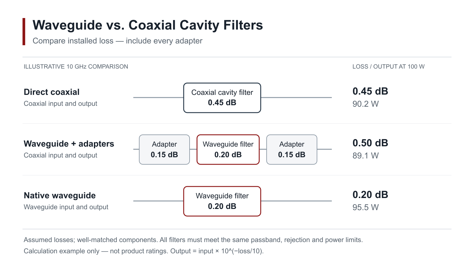
For a coaxial system, the loss of waveguide-to-coaxial adapters can outweigh the waveguide filter’s advantage. The following example assumes both filters meet the same passband, rejection, and power requirements.
| Item | Direct coaxial | Waveguide with adapters |
|---|---|---|
| Filter loss | 0.45 dB | 0.20 dB |
| Added adapter loss | 0 dB | 0.15 + 0.15 dB |
| Approximate installed loss | 0.45 dB | 0.50 dB |
| Output at 100 W input | 90.2 W | 89.1 W |
The direct coaxial option delivers about 1.0 W more, using unrounded values. In a native waveguide system, the adapters are unnecessary and the 0.20 dB filter delivers about 95.5 W. Use actual adapter specifications in the final budget; 0.15 dB is an assumption here.
Adding losses in dB is an approximation for well-matched components. Use cascaded S-parameters or measure the complete assembly when mismatch affects the result.
Connector and Flange Fit
- Coaxial connections: Confirm the impedance, gender, frequency rating, and power limits of the exact connector model. An 18 GHz connector does not extend a 9.9–10.1 GHz filter’s passband.
- Waveguide connections: Match the complete EIA or IEC flange designation, bolt pattern, alignment features, and mating face. Two WR-90 labels do not establish flange compatibility.
- Pressurized connections: Specify pressure difference, leak rate, and seal profile for the pressure and sealing components.
An SMA-equipped filter may contain a waveguide cavity with an internal transition. Ask for the internal filter type and confirm that quoted loss and power ratings apply at the external ports.
Other Acceptance Limits
Return Loss
A 20 dB minimum return-loss requirement applies across the specified passband. A 15 dB result at the edge fails even if the center reaches 25 dB. Return losses of 15 dB and 20 dB correspond to approximately 3.16% and 1% reflected power.[3]
Receiver Noise and Blocking
With the filter at 290 K and matched stages, 0.5 dB of passive loss ahead of an amplifier with a 1.0 dB noise figure gives a combined noise figure of about 1.5 dB.[4] Lower loss must still leave enough rejection: an interferer at −10 dBm needs 30 dB attenuation to reach a downstream limit of −40 dBm, or 33 dB with a 3 dB design margin.
Group Delay and PIM
For wideband modulation or short pulses, specify group-delay variation across the occupied band—for example, 9.95–10.05 GHz. Evaluate the filter’s complex S21 against the intended waveform for error vector magnitude (EVM) or pulse distortion. A single value at 10 GHz does not describe that variation.
For multicarrier systems, specify passive intermodulation (PIM) test power, carrier frequencies, measurement bandwidth, and ports. Carriers at 935 MHz and 960 MHz can generate third-order products at 910 MHz and 985 MHz. With a single-carrier reference of 43 dBm, −150 dBc equals −107 dBm; results taken at different carrier powers are not directly interchangeable.
RFQ Checklist
| Item | Example or required detail |
|---|---|
| Passband | 9.9–10.1 GHz; insertion loss ≤0.5 dB; return loss ≥18 dB throughout. |
| Stopband | Input-to-output attenuation ≥40 dB at 9.5 GHz and 10.5 GHz. Specify band limits where continuous coverage is required. |
| Power | 20 W average and 200 W peak in-band, with waveform details. State out-of-band input power and allowed load mismatch separately. |
| Interfaces and size | Connector model and gender, or waveguide and flange drawings; maximum envelope and mounting-hole positions. |
| Operating conditions | For example, −20 to +60 °C; specify cooling, pressure, and applicable environmental requirements. |
| Verification | Guaranteed limits at stated temperatures and powers; reference planes that explicitly include or exclude adapters. |
These RFQ values are examples. Confirm that the proposed design meets them simultaneously; room-temperature typical curves do not establish full-temperature or rated-power performance.